[orientation_of_real_linear_space] orientation
There are two orientations. For a basis of , swapping two vectors once changes the orientation, introducing a factor . This is similar to alternating tensors. Orientation is defined as the quotient of bases by the same orientation, equivalent to the decomposition .
Def [orientation_of_boundary_of_convex_hull]
The orientation of the oriented boundary of a convex hull is: for the affine subspace containing a facet , define an orientation such that the exterior is in the positive -dimensional direction, and the interior is in the negative -dimensional direction.
Specifically, take an orientation of (take a basis ), let lie in the -dimensional hyperplane . Let be a vector pointing from into the interior of the convex hull . Then choose a basis in the -dimensional such that is a positively oriented basis of (the linear transformation from to has positive ). This assigns a positive orientation to the -dimensional and .
One can continue to define orientations for the boundary of the boundary.
Def [oriented_simplex]
Simplex has a better way to handle orientation.
From the vertices , one can construct an oriented basis of . Denote this as .
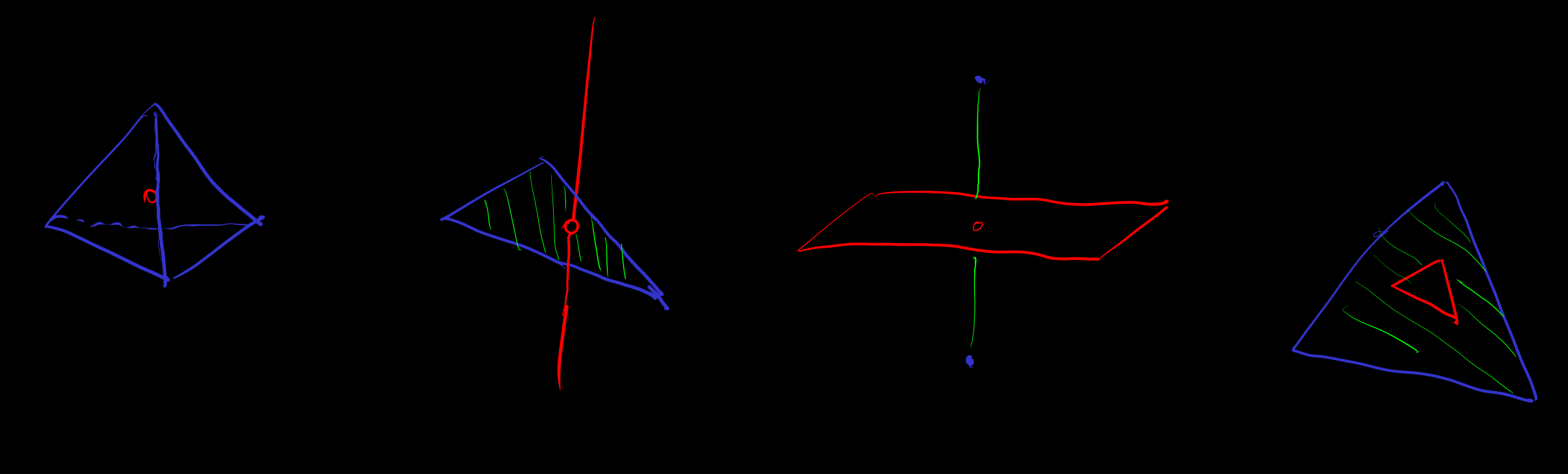
Example Tetrahedron, right-hand rule (indices of vertices in the picture start from instead of )
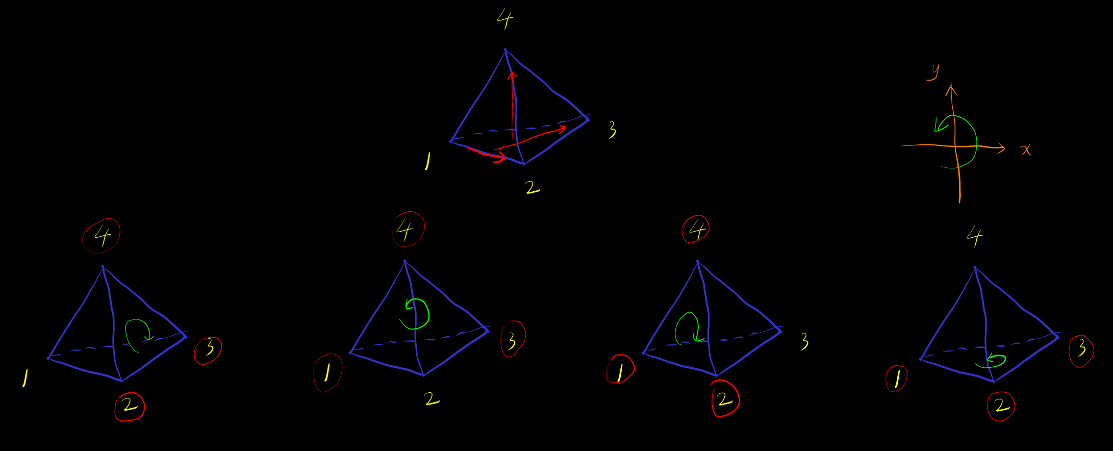
Prop [oriented_simplex_permutation] Swapping any two adjacent vertices of an oriented simplex multiplies its corresponding geometric orientation (determinant of the basis) strictly by . Consequently, for any permutation , the orientation changes by .
Proof
Let the initial path basis be , where the step vectors are .
Now we want to swap adjacent vertices and . This only affects and .
We discuss three cases:
Case 1: Swapping intermediate adjacent vertices and ()
After swapping, the local vertex sequence changes from to
The corresponding new step vectors change as follows:
Extracting these three affected columns, we observe the local transition matrix:
The determinant of this local matrix is .
Case 2: Swapping the start vertices and (i.e., )
After swapping, the sequence starts with . Only the first two step vectors are affected:
The local transition matrix is:
The determinant of this matrix is .
Case 3: Swapping the end vertices and (i.e., )
After swapping, the sequence ends with . Only the last two step vectors are affected:
The local transition matrix is:
The determinant of this matrix is .
In summary, in the path basis, swapping any adjacent vertices makes the determinant of the transition matrix strictly equal to . Thus, for any permutation , after an even/odd number of adjacent swaps, the orientation changes by .
Prop [oriented_simplex_boundary] Using the path basis combined with the geometric convention “Outward Normal FIRST”, deleting vertex results in an induced orientation coefficient of .
Proof
Let the path basis of simplex be , where the step vectors are defined as .
Now we study the -dimensional boundary after deleting . We consider three cases for its path basis and outward normal:
Case 1: Deleting an intermediate vertex ()
For , the path sequence no longer goes through , but instead takes a “shortcut” directly from to . The vector for this step is:
Thus, the path basis of merges the two original steps into one:
(Note that now has vectors, with in the -th position).
Next, find the outward normal . Since is the opposite vertex, the step from a point on to clearly points inward. Therefore, we can directly choose the outward normal .
According to the “Outward Normal FIRST” rule, prepend to to construct the geometric determinant basis:
We transform this back to the original basis via elementary column operations:
- Add the 1st column () to the -th column (). This elementary column operation does not change the determinant. After addition, the -th column becomes . The basis becomes:
- Factor out the negative sign from the 1st column, multiplying the determinant by . The basis becomes:
- Move from the 1st column back to its original -th position. It needs to pass , requiring adjacent column swaps. Each swap multiplies by , so the determinant is multiplied by .
The total determinant sign change is: .
Case 2: Deleting the start vertex (i.e., )
For , the sequence starts directly at , so its path basis loses the first step:
Find the outward normal. The vector from the new start to the old start is inward: . So the outward normal is .
The concatenated geometric determinant basis is simply:
This is exactly the original basis! Hence, no sign change, the coefficient is .
Case 3: Deleting the end vertex (i.e., )
For , the sequence ends early at . Its path basis loses the last step:
The inward vector points from to , i.e., . The outward normal is .
Concatenate the geometric determinant basis:
- Factor the negative sign from the 1st column: multiply determinant by , yielding .
- Move from the 1st column all the way to the end (-th column). It must pass the remaining vectors, requiring swaps. Multiply determinant by .
Total sign change: .
Prop [simplex_boundary_of_boundary_is_zero] For a simplex, if two -dimensional oriented boundaries share a common -dimensional boundary , then the orientations induced on by and are opposite (this is the famous in algebraic topology).
Proof
Let the two -dimensional facets be (obtained by removing ) and (obtained by removing ). Assume without loss of generality that the original indices satisfy .
Their common -dimensional face is denoted , consisting of the vertices with and removed.
We compute the orientation signs induced on from and respectively:
1. Inducing from to : The oriented sequence of itself is . In this new sequence, because (which was earlier) is removed, the actual index position of the later shifts forward by one, becoming . Therefore, when subsequently removing from to obtain , the newly induced sign coefficient must be multiplied by . The final orientation reaching is:
2. Inducing from to : The oriented sequence of itself is . In this sequence, since the removed vertex is later, it has no effect on the index position of the earlier , which remains . Hence, when subsequently removing from to obtain , the newly induced sign coefficient is simply multiplied by . The final orientation reaching is:
Conclusion: The orientation coefficient induced via the route is , while the one via the route is . Clearly . Since the underlying vertex orderings are identical, the geometric orientations strictly cancel each other out!
Def [simplex_boundary_chain]
Prop [boundary_of_simplex_boundary_chain_is_zero]
Proof
By linearity of the boundary operator, we expand it twice consecutively:
Now expand the inner carefully. For a fixed , the simplex is missing vertex and has vertices. When we subsequently remove a vertex (), we must account for how the absence of changes the absolute index of in the new sequence:
-
Case 1:
appears before . Removing does not affect the position of ; its index in the new sequence remains . The resulting term is: .
-
Case 2:
appears after . Because the earlier has been removed, the index of in the new sequence shifts forward by one, becoming . The resulting term is: .
Substitute these two cases back into the double sum:
Observe that both double sums range over the same set of index pairs: all pairs with . To see the cancellation clearly, perform a dummy variable substitution in the first sum: let , so . In the second sum, let , again .
Substituting the renamed variables:
Since the exponents and differ by exactly , the terms and are opposite in sign and sum strictly to .
Therefore every term cancels perfectly, and the final result is .
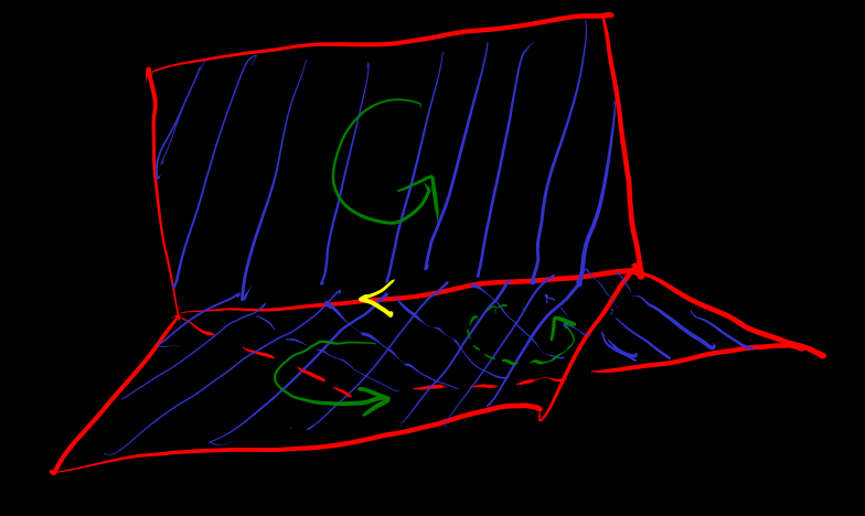
[orientable_low_dim_polyhera] A polytope orientability is defined as: when constructing a polytope using hulls, one can define compatible orientations for all -hulls such that for two adjacent -hulls , the orientation of their common -dimensional boundary hull is compatible, i.e., orientation corresponds to the interior of and the exterior of . Orientation corresponds to the interior of and the exterior of .
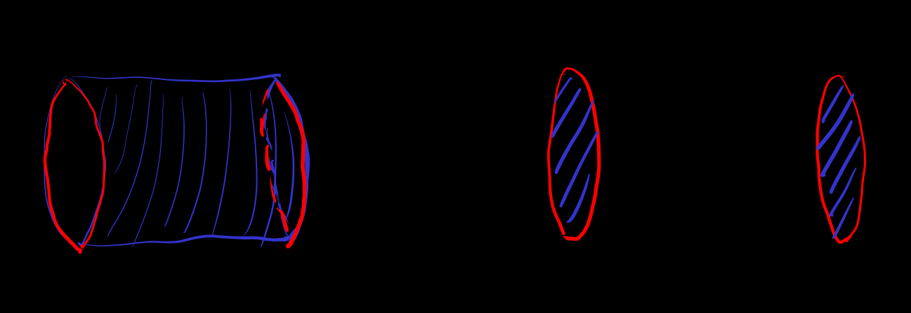
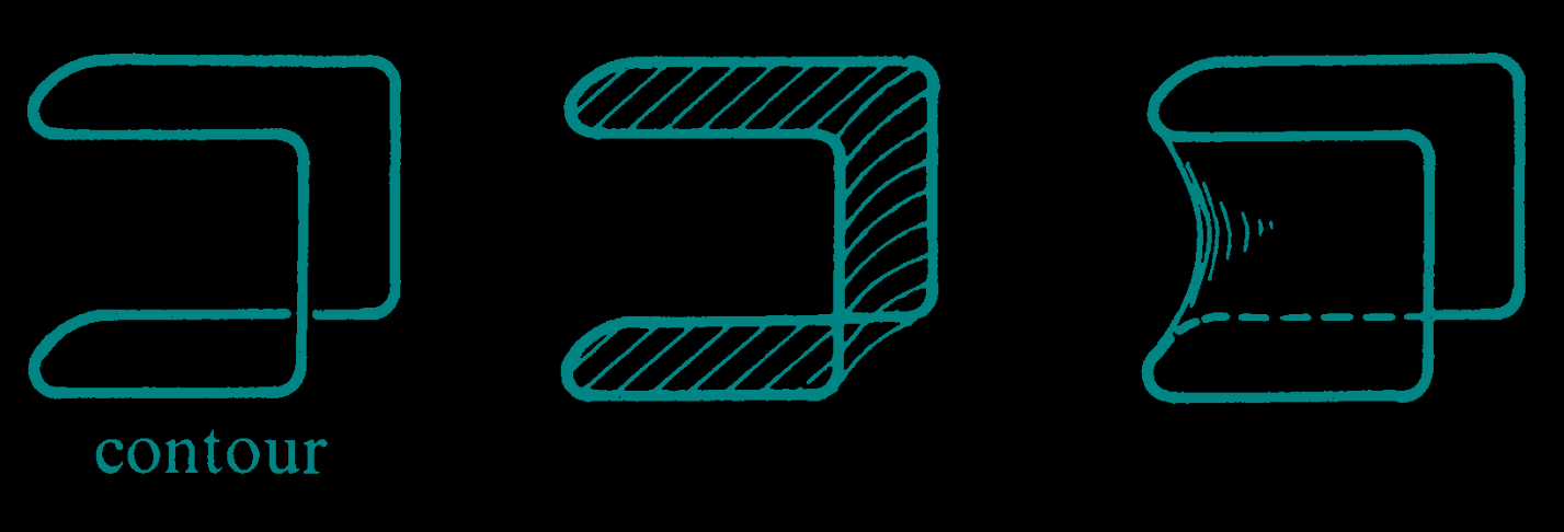
Example [Mobius_strip] Non-orientable Möbius-type polytope (image modified from wiki)

No matter how one defines the orientation for each -hull, there exists a pair of adjacent -hulls whose common -dimensional boundary hull has incompatible orientations.
Constructively, starting from an initial -hull and repeatedly defining compatible orientations for adjacent -hulls, going around a loop leads to an incompatibility on the boundary hull: orientation would correspond to the interior of both and , while orientation would correspond to the exterior of both and .
[hull_chain] . Due to geometric meaning, we only consider coefficients here.
A hull chain can be represented as a simplex chain.
[boundary_operator]
Boundary operator
is a cycle :=
is a boundary :=
or
or
Example
-
boundary-op-not-injective (p. 405 of ref-11, vol.1)
-
[tri_intersect_boundary]
[homology]
k-th homology
where are subspaces of the -chain space.
[real_linear_space_trivial_homology]
() is simplicially homology trivial: or or in , the boundary of is zero <==> is a boundary.
That is, for a -dimensional simplex chain , if its boundary , then must be a boundary, i.e., there exists a -dimensional simplex chain such that .
For , the equivalent algebraic statement for trivial homology requires an additional reduced condition — namely, the sum of coefficients of the -chain is .)
For , intuitively, if an -dimensional simplex chain has zero boundary , then .
Proof
Consider first the cases ; the case will be treated afterwards.
1. Cone Operator
Arbitrarily choose a reference point in as the cone apex.
For any -dimensional simplex , define its cone with respect to as , which is a -dimensional simplex formed by prepending to the vertex sequence:
For a -chain which is a finite linear combination of simplices, extend this operator linearly:
2. Algebraic Boundary Identity for the Cone (Chain Homotopy)
Now compute using the definition:
Remove each vertex sequentially from this -dimensional sequence:
-
When removing the vertex at position (i.e., ), the coefficient is , and the remaining sequence is exactly the original :
-
When removing the vertex at position (which is from the original ), the coefficient is . The sum over these terms is:
Factor out a from :
The expression inside the parentheses is precisely . Thus, this term equals .
Combining these two parts yields a symmetric and elegant identity:
Since the boundary operator and the cone operator are linear, this identity also holds for any chain :
3. Proving Triviality
If satisfies (when ), substitute into the above identity, obtaining:
Let . We have algebraically constructed a -chain such that , proving homology triviality.
(Remark: For , a -chain , we have . For to hold, the algebraic reduced condition is necessary.)
4. Supplementary Discussion on Affine Independence and Non-degenerate Simplices
By the strict definition of a simplex, its vertices must be affinely independent. The above algebraic derivation remains consistent with this geometric constraint:
When : The chain consists of only finitely many -simplices, whose affine subspaces have dimension at most . Since , the union of finitely many proper -dimensional subspaces cannot cover all of . Therefore, we can always choose a point in such that does not belong to the affine subspace of any . This guarantees that the newly added is affinely independent from the vertices of each , and the generated consists entirely of strictly legal, non-degenerate simplices.
The case
If is regarded as a formal chain, is false; but if is regarded as a “signed geometric coverage (multiplicity)” of space, then its geometric sum is indeed zero everywhere.
- Algebraically
(Example in ): Take three distinct points on a line. Any two points are affinely independent, thus forming legal -simplices. Define a -coefficient -chain: . Then , but algebraically .
Higher-dimensional generalization: In , choose points in general position, i.e., any of them are affinely independent. Any selection of points forms a legal -simplex. Let . By a similar alternating cancellation principle as in simplex_boundary_of_boundary_is_zero, we have and .
- Geometrically
Although the formal combination is non-zero, if we interpret the -chain as a signed coverage weight function on , i.e., a point accumulates weight when it lies in the , we prove: when , the corresponding spatial superposition weight is zero everywhere.
For any point in in general position (not lying on any low-dimensional boundary of the ), we show that the weight at is .
Draw an arbitrary ray from : . Since all are bounded convex hulls, as , the ray must eventually exit all simplices, where the external coverage weight is strictly .
Now walk backwards along the ray from to . The coverage weight of space only changes when the ray crosses the hyperplane containing an -dimensional facet of some simplex.
The weight step from entering or exiting a simplex is completely determined by the induced orientation of that facet and the coefficient .
The algebraic premise means the sum of coefficients of all oriented -dimensional faces forming is strictly . Specifically, on any local hyperplane , the signed coefficients of adjacent -simplices contributing to that -dimensional face must perfectly cancel the step incurred when crossing .
Since the total weight change when the ray crosses any boundary satisfies , and the initial weight at is , walking backwards along the ray to the starting point shows that the total superposed weight at must be identically .
Thus, from the perspective of geometric entities, the region represented by the chain is indeed completely canceled to zero by positive and negative contributions.
Prop [uniqueness_of_n_hull_chain_with_boundary]
Proof
[homology_hole] For the set minus a finite or countable number of disjoint linear subspaces or polytopes, the homology is not zero.
[Stokes_theorem]
Analogous to the one-dimensional Fundamental Theorem of Calculus. Intuitively, divergence and the divergence theorem = the higher-dimensional Fundamental Theorem of Calculus.
Define in coordinates the [exterior_differential] , where is the coordinate volume, and the result is independent of the coordinate choice.
Then we have Stokes’ theorem.
For an orientable analytic manifold with boundary and an -form :
or .
If one uses a box in coordinates to compute , partial derivatives of certain quantities along coordinate directions will appear. The result will be:
However, in the proof of the one-dimensional Fundamental Theorem of Calculus, the partition of the interval, the boundary of the interval, and the integral over the boundary of the interval all rely on the simplicity of being “straight”. Higher-dimensional regions can be “curved”, making the situation more difficult.
[Stokes_theorem_simple] For higher dimensions, one can first handle straight objects, i.e., simplices/hulls/parallelotopes. Partitions using the same type of regions work, and boundary cancellation is simple. Then, analogous to the one-dimensional case, one can use the mean value theorem for approximation combined with compactness control. This proves Stokes’ theorem for simplices/hulls/parallelotopes in .
[Stokes_theorem_proof] Question
Following the intuitive handling of integration on manifolds and Stokes’ theorem, one should consider directly partitioning the manifold.
Partitions in integration can directly use zero-order measurable sets (closed under diffeomorphisms), but this is too coarse to control the boundary. The regions used for partitioning in Stokes’ theorem should be sets of finite perimeter (Caccioppoli sets) from geometric measure theory (ref_33), which are expected to be closed under finite unions, intersections, and differences, and also closed under diffeomorphisms.
Prove that a manifold with boundary is locally such a set (find a polyhedral approximation using manifold properties), and that the integral over the boundary in this theory coincides with the integral over the boundary in manifold theory (similar to the reduced boundary theory in geometric measure theory). Prove that well-behaved manifolds with singularities (e.g., polytopes, cones, well-behaved singularities of codimension ) also belong to such sets.
The proof of Stokes’ theorem would then be: finitely cover the compact support of the form with such regions, subtract overlaps, partition, apply Stokes’ theorem on the partitioned regions, cancel integrals on interior boundaries, leaving only the genuine boundary of the manifold.
Although I wish to avoid compactly supported smooth forms, some care is needed. The strict inclusions on suggest that (local) Sobolev or absolute continuity of an -form and its exterior derivative, lacking a mean value theorem, is not suitable for geometrically defining the exterior derivative as the limit of boundary integral over volume and then using the mean value theorem and barycentric subdivision to geometrically prove that simplices satisfy Stokes’ theorem. Sobolev or absolute continuity still implies that each sufficiently small local simplex satisfies Stokes’ theorem. If boundedness is added to the exterior derivative, then the mean value theorem can indeed be used for control. However, the mean value theorem essentially defines Lipschitz continuity (with respect to simplex volume), and mere (local) Lipschitz continuity will also imply almost everywhere existence of the derivative which is (locally) .
The meaning of an -form. As long as a -dimensional affine subspace is viewed as a manifold (e.g., choose a -basis to establish coordinates), it has its own volume. After choosing a basis for the -subspace, a pointwise-defined -form on becomes a real-valued function on it. Integrability over the boundary of any simplex requires that the -form become an integrable function in every -direction. By linearity of forms and integration, it suffices that its components become integrable functions with respect to a basis of the space of -directions (corresponding to the -alternating tensor space on ), i.e., that the “components of the -form on are locally “. Such forms are preserved under diffeomorphisms, just as Lebesgue measurable sets are. In principle, one can say that the real-valued function induced by a -form on a -subspace in each -direction can be approximated by piecewise constant functions supported on simplices, in the sense of the usual integral of an -form on . Without assuming differentiability, we haven’t even defined the exterior derivative, nor proven Stokes’ theorem on simplices.
Attempt to define differentiation starting from integration, as a way to combine measure theory and differentials. First, define what it means for an -form to satisfy a local infinitesimal Stokes’ theorem — an integrable version of an exterior-differentiable form — then use polyhedral approximations of forms satisfying the local infinitesimal Stokes’ theorem on simplex regions to define what it means for a region to globally satisfy Stokes’ theorem.
Then define the exterior derivative of an -form using the average derivative .
Next, one needs to prove Stokes’ theorem for simplices. Using barycentric subdivision techniques, the proof for smooth forms uses estimates provided by the mean value theorem.
Then one can attempt to define “regions where Stokes’ theorem holds”, similar to sets of finite perimeter. The required restrictions are, intuitively, that among all measurable sets, some possess boundary properties allowing the global Stokes’ theorem. Intuitively, the restriction conditions for such regions should be similar to the existence of a subnet in the net of approximating polytopes that well-uniformly controls the integrals of all normalized or projected integrable exterior-differentiable forms (or something more general) on the boundaries of the approximating polytopes.
The relationship between functions of bounded variation and sets of finite perimeter in geometric measure theory is analogous to the relationship between integrable functions and measurable sets in zero-order measure theory.
Since exterior differentiation involves only first-order derivatives, not infinite-order derivatives, the norm of a form on a metric manifold is suitable for Banach/Hilbert space theory (infinite-order derivatives are not suitable for Banach space theory).
Because the topology of a manifold may have non-trivial homology, some cohomologically non-zero forms may have an exterior derivative whose integral cannot be fully canceled by interior boundaries, leading to an additional “residue” similar to complex analysis. For example, [cohomology_hole] Example in , or , satisfies , so its integral over is zero, but the integral of over the boundary of is non-zero. Example has homology isomorphic to .
Another example where boundary cancellation fails in integration: a vector field or form that satisfies Stokes’ theorem on a closed ball may no longer satisfy it after removing a region similar to a closed disk from the interior of . Intuitively, after removing a closed disk, the flux leaks out, indicating that the new boundary does not enclose the manifold’s interior. If an open disk is removed instead of a closed one, the result is not a manifold with boundary; it has a boundary of codimension , and the boundary of that boundary is not zero.
One might need to consider some compactness constraint, as non-compactness can introduce some kind of failure of boundary cancellation due to infinity, potentially resulting in a residue term relative to infinity.
I have not handled Stokes’ theorem for manifolds without boundary, nor defined . Example of a manifold without boundary: .
Given counterexamples like the Cantor set, almost-everywhere analyticity is not the correct way to handle singularities.
Correspondence between boundary operator and exterior derivative.
Homology.
Cohomology.
[coboundary_operator]
Coboundary
Cocycle . Intuitively, the divergence of the form at a point is zero.
or . Intuitively, the divergence field is divergence-free.
or
[de_Rham_cohomolgy] k-th de Rham cohomology
in , cohomology trivial
The case of metric manifolds
The integral of the form is equivalent to the integral of
[Hodge_star]
Hodge star operator as the orthogonal complement dual of the form
with ==>
==>
[flux]
Integral of form -> Integral of -> Integral of , interpreted as the quantity of the orthogonal complement of integrated over , i.e. flux
Represent the flux alternating tensor using the inner product duality , the inner product represents the orthogonal projection of the quantity onto the flux direction (image)
Example in Euclidean , .
- form
Coordinates
Stokes’ theorem [gradient]
- form
Note that at this time, you can add a directional two-dimensional “rotation 90 degrees” to change the two-dimensional divergence into a two-dimensional curl, and the normal flux to the boundary becomes the tangent flow to the boundary.
Coordinates
Stokes’ Theorem [curl]
where
- form
Coordinates
Stokes’ Theorem [divergence]
in Minkowski ,