note-math

Consider the subspace

The following are equivalent

• not co-linear

if , according to the intuition of (draw a picture), bases of the following types are all possible

• 2 time(-like)
• 2 space
• 1 time, 1 space
• 1 time, 1 light
• 1 space, 1 light
• 2 light

Example

• 2 time(-like)
  

  , where
  
  can linearly generate , thus spanning
• 2 space
  , where
• 1 time, 1 space
  
• 1 time, 1 light
  
• 1 space, 1 light similarly
• 2 light
  Example . Note .
  generate

Consider a general in

[signature-of-2d-subspace-of-spacetime] Prop The possible signatures of a in Minkowski are

We will prove later that signatures are impossible

Intuitively, the plane spanned by two lines (imagine the case of )

• intersects both the interior and exterior of the light cone. Although all types of bases are possible, all bases of the following types are of signature

  • 2 time
  • 1 time, 1 light
  • 2 light

• only intersects the exterior of the light cone

  • 2 space

• is tangent to the light cone, does not intersect the interior of the light cone, and intersects the light cone only along a single light-like line

  • 1 light, 1 space

Prop can have signature subspaces. Proof ‘s

Prop time-like is orthogonal only to space-like

let be time-like. Using orthogonal decomposition , let then ==> is space-like

Prop light-like is not orthogonal to

• time-like. because time-like is orthogonal only to space-like
• light-like vectors other than those colinear with itself [metric-cannot-distinguish-colinear-light-like]

Proof

Prop The signature of a two-dimensional subspace of cannot be or

Proof Use the previous theorem

Question Is there a proof that does not rely on orthogonal decomposition of time and space? But note, this proposition does not hold for general . In , the following are orthogonal and non-collinear

• 1 time, 1 light
• 2 light

A further concept is “Totally Isotropic Subspace”

Prop When , all signatures are possible for the subspace of

Proof In this case contains the subspace , where it is easy to construct subspaces of all possible signatures

Prop For two non-collinear time-like vectors in , the signature of their span is

Proof Use one of the time-like vectors as the initial basis to generate an orthogonal basis for , but the signature cannot be , so it must be

Prop In let be light-like, be time-like or light-like, and be non-collinear. Then

Proof

[simultaneity-relativity] Relativity of Simultaneity

Take a spacetime orthogonal decomposition of

Prop ==> The sign of the product of time components determines the sign of the inner product

Proof Case analysis for

• . let . . Similarly for . Then by the Euclidean inner product inequality

  Thus , i.e., same sign as

• . let . Set and apply the conclusion from

in Euclidean, we have

Inner product inequality ==> Triangle inequality

in signature quadratic form, this generally does not hold

As mentioned earlier, the quadratic form under the basis corresponds to the matrix . Transforming to the standard quadratic form, the corresponding matrix transformation is

[quadratic-form-inequality-Minkowski] Inner product inequality

• 
  one positive and one negative, corresponding to signature
• 
  with the same sign, corresponding to or signature
• 
  Other signatures or are collinear

[triangel-inequality-Minkowski] signature triangle inequality

Proof of 2 time-like

The limit or continuity in Euclidean space is directly defined using open balls (to simplify the discussion, only consider the origin as the center)

In Minkowski space or p,q quadratic form space, a direct imitation of the Euclidean case is

• timelike , spacelike , or
• When merging classes, the class is empty

But note that at this time

1. The limit meaning represented by is different from the Euclidean case. For example, although two distinct points on the light cone are “separated,” their quadratic distance is zero. For a point on the light cone, although it is separated from , it can be transformed via so that the coordinates of approach arbitrarily. Taking as an example, let . After transformation, , then . under the orbit of the action is the ray
2. Taking as an example, should be the analogue of the sphere in . Based on graphical intuition in , some points on appear far from the origin , but in fact the distance of any point on is the same; any two points on can be transformed into each other via an transformation, just like the situation with . On , when the quadratic form distance , it can be considered as the timelike geodesic distance or the proper time of an inertial particle. Timelike points on can be transformed via to have zero spatial coordinates, meaning transforming from uniform motion to rest, where proper time = time. Similar conclusions likely hold for as well.

“Fortunately”, the “continuity of coordinate distance” in , i.e., the product distance of , implies the “continuity of quadratic form distance” in , because , and further implies differentiability/analyticity.

Conversely, in the case of non-Euclidean geometry, continuity of the quadratic form distance does not imply continuity of the coordinate distance.

When dealing with objects in Minkowski space , many useful functions are also “continuous or analytic with respect to spacetime coordinate distance”, i.e., continuous or analytic under the product distance in one coordinate.

When dealing with differentiability/analyticity, since dividing by may be encountered in the direction of the light cone in the domain or codomain, those points are generally considered to be differentiable/analytic.

However, there may exist useful functions that are continuous/analytic under the quadratic form distance but not continuous/not analytic under the spacetime coordinate distance.

Possible clue for the rationality of the quadratic form distance: , via the tensor as a linear map space, inherits a tensor quadratic form. When restricted to , it becomes proportional to the Killing form quadratic form of Killing-form-of-orthogonal-group. Signature , where is the number of boosts, are time-like rotations, and are space-like rotations. Under the Killing form, boosts have positive distance, while time/space rotations both have negative distance.

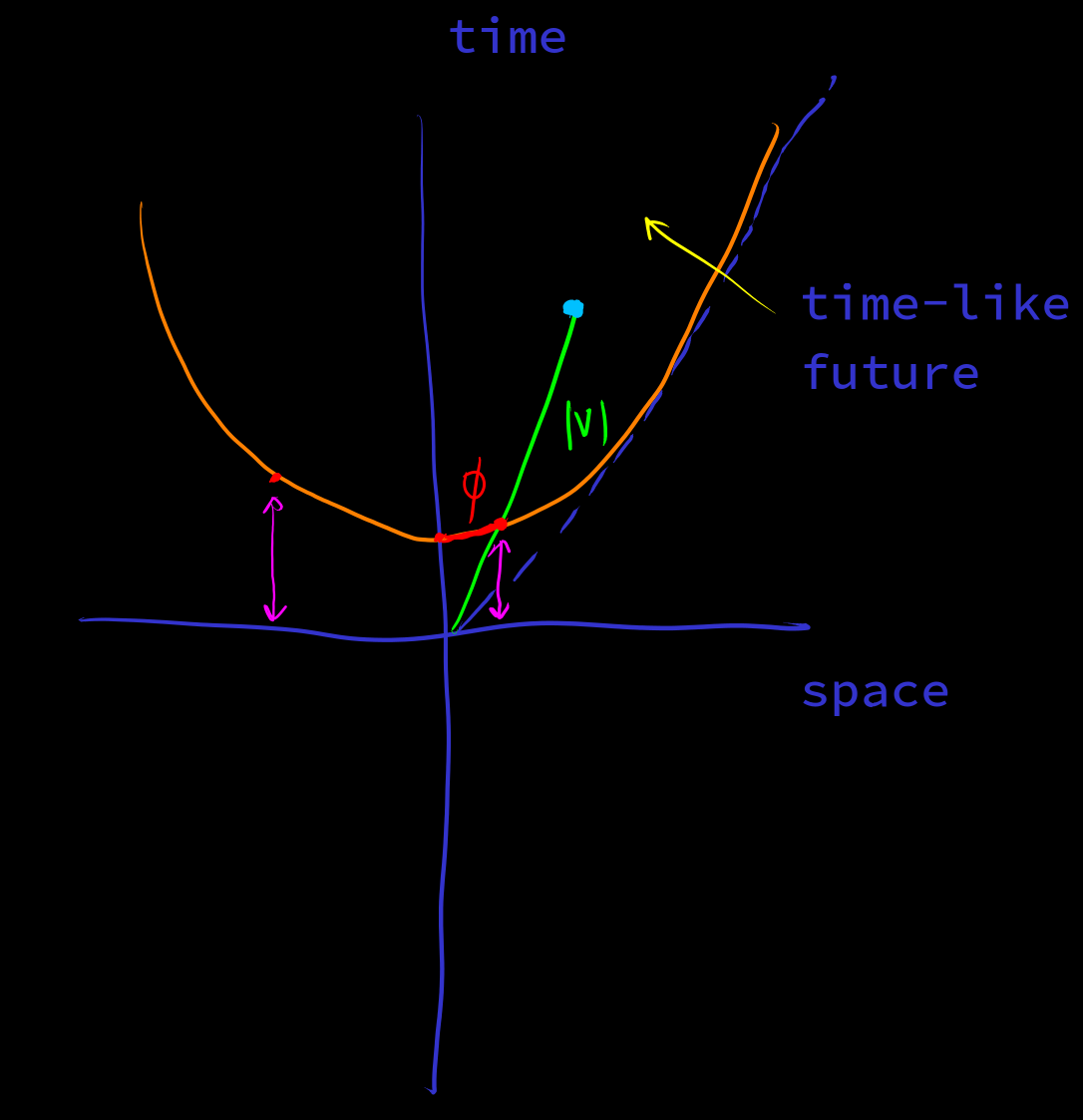
‘s timelike region . It can be decomposed into the radial space part and the directional space part

Similar to polar coordinates in , we can use hyperbolic polar coordinates , where is the quadratic form distance, and is the geodesic length on , also called the hyperbolic angle [hyperbolic-angle] or rapidity [rapidity]

[polor-coordinate-hyperbolic] Hyperbolic polar coordinates

[hyperbolic-cosine-formula] Hyperbolic Cosine Formula

[isom-top-hyperbolic-Euclidean]

Limit structure of under the distance geodesic distance Euclidean

Proof

Generalize to , Euclidean

Proof

Geodesics on quadratic manifolds can be defined using purely quadratic form techniques

The tangent space at point of the quadratic manifold can be defined as the (affine) subspace orthogonal to the radial vector

The initial direction of the geodesic starting from point is in the tangent space of at point ,

The geodesic is defined as

type (p. 19 of ref-9)

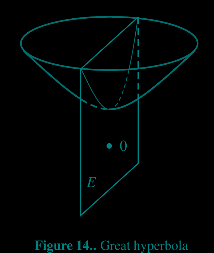
type

is a Riemann manifold with constant negative curvature

is a Lorentz manifold with constant positive curvature

alias de Sitter space

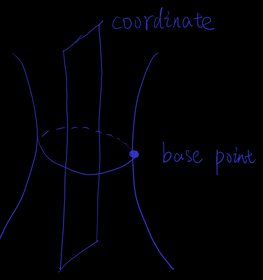
The base points (“north and south poles”) of the stereographic projection of the sphere lie on . More than two coordinate charts are needed to cover the entire

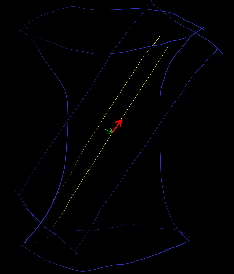
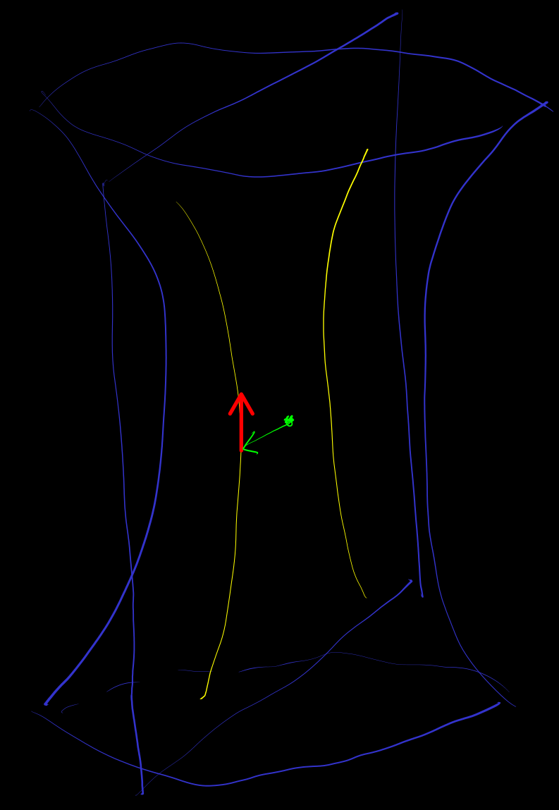
[stereographic-projective-hyperbolic] For the time-like hyperboloid , consider stereographic projection. The two base points lie on the two sheets of the hyperboloid respectively, and the projection forms separated singularities in the light cone direction (the cross shape in the figure below)

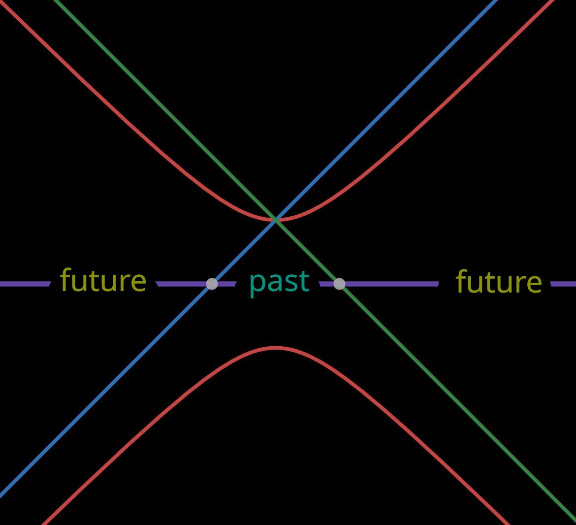
In the projection coordinates of the future base point, the coordinates of the past base point are zero, but the coordinates of the future base point are either absent or are

is special, so the future coordinates in the figure above are disconnected. However, when the spatial dimension is , the future coordinates should be connected

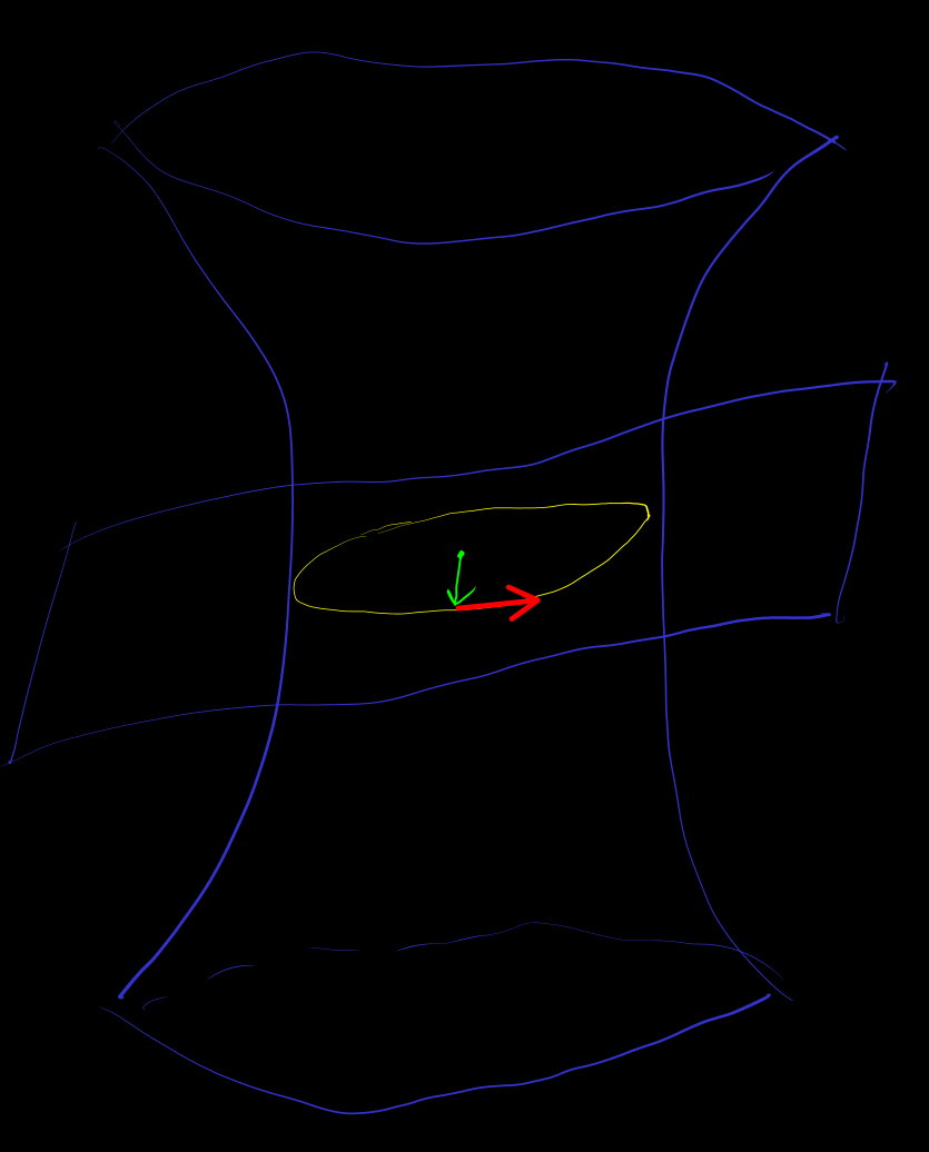
For the space-like hyperboloid, use space-like base points to define the hyperbolic projection. The projection coordinate chart is a Minkowski space of one lower dimension

Perform a 3D plot for the case of , drawing the light cone of the base point (note that the light cone is “vertical”)

Even if the visual intuition for plotting might be difficult, the analytical calculation should not be hard