note-math

The power function order in the power series $\sum_{0 . . \infty} 𝑎_{𝑛} 𝑣^{𝑛}$ is different, introducing the asymmetry of the coefficient $𝑎_{𝑛}$ , which makes it not necessarily suitable for series rearrangement? Although we will still discuss absolute convergence

One-dimensional case begins

#link(<geometric-series>)[Geometric series]

| 𝑎 | < 1 ⟹ \sum_{𝑛 \in ℕ} 𝑎^{𝑛} = lim_{𝑛 \to \infty} \frac{1 - 𝑎^{𝑛 + 1}}{1 - 𝑎} = \frac{1}{1 - 𝑎}

in $𝕂$ , $| 𝑎 𝑏 | = | 𝑎 | | 𝑏 |$

$| 𝑎_{𝑛} 𝑣^{𝑛} | = {(| 𝑎_{𝑛} |^{\frac{1}{𝑛}} | 𝑣 |)}^{𝑛}$

convergence-radius-1d_(tag) Radius of convergence

(cf. #link(<limsup>)[])

\begin{matrix} 𝑅 & ≔ & \frac{1}{\underset{𝑛 \to \infty}{lim sup} {| 𝑎_{𝑛} |^{\frac{1}{𝑛}}}} \in [0, \infty] \\ or \frac{1}{𝑅} & ≔ & \underset{𝑛 \to \infty}{lim sup} {| 𝑎_{𝑛} |^{\frac{1}{𝑛}}} \end{matrix}

==> $| 𝑎_{𝑛} |^{\frac{1}{𝑛}} \leq \frac{1}{𝑅}$

absolute-convergence-analytic-1d_(tag)

$| 𝑣 | < 𝑅$ ==> $𝑎_{𝑛} 𝑣^{𝑛}$ absolutely converges

Proof

use #link(<geometric-series-test>)[geometric series test] and $| 𝑎_{𝑛} 𝑣^{𝑛} |^{\frac{1}{𝑛}} = | 𝑎_{𝑛} |^{\frac{1}{𝑛}} | 𝑣 | \leq \frac{| 𝑣 |}{𝑅} < 1$

| \sum_{𝑛 \in ℕ} 𝑎_{𝑛} 𝑣^{𝑛} | \leq \sum_{𝑛 \in ℕ} {(\frac{| 𝑣 |}{𝑅})}^{𝑛} = \frac{1}{1 - \frac{| 𝑣 |}{𝑅}}

$| 𝑣 | > 𝑅$ ==> $𝑎_{𝑛} 𝑣^{𝑛}$ absolutely diverges

Proof $\frac{1}{𝑅} ≔ \underset{𝑛 \to \infty}{lim sup} {| 𝑎_{𝑛} |^{\frac{1}{𝑛}}}$ ==> for infinite terms in $𝑛 \in ℕ$ , $| 𝑎_{𝑛} |^{\frac{1}{𝑛}} \approx \frac{1}{𝑅} ⟹ | 𝑎_{𝑛} |^{\frac{1}{𝑛}} | 𝑣 | > 1 ⟹ | 𝑎_{𝑛} 𝑣^{𝑛} | > 1$

uniformaly-absolutely-convergence-analytic_(tag)

use $| 𝑣 | \leq 𝑟 < 𝑅$ . use #link(<geometric-serise-test>)[geometric series control]

in the closed ball $\bar{𝔹} (𝑟)$ with radius $𝑟 < 𝑅$ , $\sum 𝑎_{𝑛} 𝑣^{𝑛}$ uniformly absolutely converges

Polynomial function $𝑣 ⇝ \sum_{𝑛 = 0}^{𝑁} 𝑎_{𝑛} 𝑣^{𝑛}$ is a continuous function

Function defined by power series within the radius of convergence

$𝑣 ⇝ 𝑓 (𝑥 + 𝑣) = \sum_{𝑛 \in ℕ} 𝑎_{𝑛} 𝑣^{𝑛}$ , $| 𝑣 | < 𝑅$

analytic-imply-continuous_(tag)

$𝑅 > 0$ ==> continuous

$\begin{matrix} | 𝑓 (𝑥 + 𝑣) - 𝑓 (𝑥) | & = & | \sum_{𝑛 = 0}^{\infty} 𝑎_{𝑛} 𝑣^{𝑛} - 𝑎_{0} | \\ \leq & \sum_{𝑛 = 1}^{\infty} {(\frac{| 𝑣 |}{𝑅})}^{𝑛} \\ = & \frac{1}{1 - \frac{| 𝑣 |}{𝑅}} - 1 \end{matrix}$

$lim_{𝑣 \to 0} \frac{1}{1 - \frac{| 𝑣 |}{𝑅}} - 1 = 0$

Extending the #link(<change-base-point-polynomial>)[] of polynomials to series

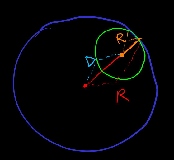
change-base-point-analytic_(tag)

$𝑅 > 0$

==> The power series after switching the base point of the power series $\sum 𝑎_{𝑛} 𝑣^{𝑛}$ to $𝑥 + Δ \in 𝔹 (𝑥, 𝑅)$

𝑓 ((𝑥 + Δ) + 𝑣) = \sum_{𝑚 \in ℕ} (\sum_{𝑛 = 𝑚}^{\infty} 𝑎_{𝑛} (𝑥) (\binom{𝑛}{𝑚}) Δ^{𝑛 - 𝑚}) 𝑣^{𝑚} = \sum_{𝑚 \in ℕ} 𝑎_{𝑚} (𝑥 + Δ) 𝑣^{𝑚}

There is also a non-zero radius of convergence $𝑅^{'} > 0$ at $𝑥 + Δ$ . (Figure) According to the triangle inequality, $𝑅^{'} \geq 𝑅 - | Δ |$

Example

$log (1 - 𝑧) \sim \sum \frac{1}{𝑛} 𝑧^{𝑛}$ 的 radius of convergence is $1$
$𝑒^{𝑧} \sim \sum \frac{1}{𝑛!} 𝑧^{𝑛}$ 的 radius of convergence is $\infty$

Convergence problem on the boundary

$log (1 - 𝑥) \sim \sum \frac{1}{𝑛} 𝑥^{𝑛}$ 的 radius of convergence is $1$ , at $𝑥 = 1$ it is the harmonic series $\sum \frac{1}{𝑛}$ , absolutely divergent
$\sum \frac{1}{𝑛^{2}} 𝑥^{𝑛}$ 的 radius of convergence is $1$ , at $𝑥 = 1$ absolutely converges to
$\sum \frac{1}{𝑛^{2}} = \frac{𝜋^{2}}{6}$
Absolute convergence vs convergence: $log (1 - 𝑥) \sim \sum \frac{1}{𝑛} 𝑥^{𝑛}$ converges at $𝑥 < 1$

Now consider the higher-dimensional case. $𝕂^{𝑑} \to 𝕂^{𝑑^{'}}$ power series

Note the $| 𝑣 |$ symmetry, for example $O (𝑑)$ of $ℝ^{𝑑}$ , $U (𝑑)$ of $ℂ^{𝑑}$

Generalize the polynomial function #link(<polynomial-function>)[] to the power series $\sum 𝐴_{𝑛} (𝑣^{𝑛})$

Unlike one-dimensional, in higher dimensions, generally there is no $| 𝐴_{𝑛} (𝑣^{𝑛}) | = | 𝐴_{𝑛} | | 𝑣 |^{𝑛}$ . There isn't even a definition for $| 𝐴_{𝑛} |$

linear-map-induced-norm_(tag)

let $𝐴 \in Lin (\otimes^{𝑛} 𝕂^{𝑑} \to 𝕂^{𝑑^{'}})$

$| 𝐴 |$ is defined as the uniform control coefficient for all directions $𝑣 \in {𝕂 ℙ}^{𝑑 - 1}$ . compactness of ${𝕂 ℙ}^{𝑑 - 1}$ will make this definition meaningful (and cannot be directly used for general $𝑝, 𝑞$ quadratic form direction space $ℚ^{𝑝, 𝑞} (\pm 1)$ )

| 𝐴 | ≔ \sup_{𝑣 \in {𝕂 ℙ}^{𝑑 - 1}} | 𝐴 (𝑣^{𝑛}) |_{𝕂^{𝑑^{'}}} = \sup_{𝑣 \in 𝕂^{𝑑}} \frac{| 𝐴 (𝑣^{𝑛}) |}{| 𝑣 |^{𝑛}}

so that (for all direction)

| 𝐴 (𝑣^{𝑛}) | \leq | 𝐴 | | 𝑣 |^{𝑛}

and

$| 𝜆 𝐴 | = | 𝜆 | | 𝐴 |$
$| 𝐴 + 𝐵 | \leq | 𝐴 | + | 𝐵 |$

Compared to the $𝕂^{1}$ case, the computability of the definition of $𝕂^{𝑑}$ is low

convergence-radius_(tag) radius of convergence

𝑅 = \frac{1}{\underset{𝑛 \to \infty}{lim sup} {| 𝐴_{𝑛} |^{\frac{1}{𝑛}}}}

absolute-convergence-analytic_(tag)

#link(<absolute-convergence-analytic-1d>)[same as] $𝕂^{1}$

$| 𝑣 | < 𝑅$ ==> $𝐴_{𝑛} (𝑣^{𝑛})$ absolutely converges
There exists a direction $\frac{𝑣}{| 𝑣 |}$ , forall $| 𝑣 | > 𝑅$ , $𝐴_{𝑛} (𝑣^{𝑛})$ is absolutely divergent

Proof (of divergence)

use #link(<linear-map-induced-norm>)[] $| 𝐴_{𝑛} |$ , there exists $𝑣_{𝑛} \in {𝕂 ℙ}^{𝑑 - 1}$ such that $| 𝐴_{𝑛} ({(𝑣_{𝑛})}^{𝑛}) | \approx | 𝐴_{𝑛} |$

use $lim sup$ definition, for infinitely many terms $𝑛 \in ℕ$ , $| 𝐴_{𝑛} |^{\frac{1}{𝑛}} \approx lim sup {| 𝐴_{𝑛} |^{\frac{1}{𝑛}}} = \frac{1}{𝑅}$

use passing to compact ${𝕂 ℙ}^{𝑑 - 1}$ and the subsequence of $𝑣_{𝑛}$ converges to $𝑣$

==> for infinitely many terms $𝑛 \in ℕ$ , $| 𝐴_{𝑛} ({(𝑣_{𝑛})}^{𝑛}) | \approx | 𝐴_{𝑛} (𝑣^{𝑛}) |$

==> for infinitely many terms $𝑛 \in ℕ$ , $| 𝐴_{𝑛} (𝑣^{𝑛}) |^{\frac{1}{𝑛}} \approx lim sup {| 𝐴_{𝑛} |^{\frac{1}{𝑛}}} = \frac{1}{𝑅}$

Scale $\frac{𝑤}{| 𝑤 |} ≔ 𝑣 \in {𝕂 ℙ}^{𝑑 - 1}$ to $𝑤 \in 𝕂^{𝑑}$

==> $| 𝐴_{𝑛} (𝑤^{𝑛}) | = | 𝐴_{𝑛} (𝑣) | | 𝑤 |^{𝑛}$

let $| 𝑤 | > 𝑅$

==> for infinitely many terms $𝑛 \in ℕ$ , $| 𝐴_{𝑛} |^{\frac{1}{𝑛}} | 𝑤 | > 1 ⟹ | 𝐴_{𝑛} (𝑤^{𝑛}) | > 1$

Another point of view: for each direction $𝑣 \in {𝕂 ℙ}^{𝑑 - 1}$ , consider the radius of convergence $𝑅 (𝑣)$ of the $𝕂$ line embedding. then let $𝑅 = \inf_{𝑣 \in {𝕂 ℙ}^{𝑑 - 1}} 𝑅 (𝑣)$

Similar to one-dimensional case also have

#link(<uniformaly-absolutely-convergence-analytic>)[]
#link(<analytic-imply-continuous>)[]
#link(<change-base-point-analytic>)[]

for $𝑓 (𝑥 + 𝑣) = \sum 𝐴_{𝑛} (𝑣^{𝑛})$ , the $𝑛$ -th order #link(<difference-polynomial>)[difference] gives

𝑛! 𝐴_{𝑛} (𝑣_{1} \dots 𝑣_{𝑛}) + 𝑜 (𝑣^{𝑛})

Replace $𝑣_{𝑘} \to 𝑡_{𝑘} 𝑣_{𝑘}$

𝑡_{1} \dots 𝑡_{𝑛} 𝑛! 𝐴_{𝑛} (𝑣_{1} \dots 𝑣_{𝑛}) + 𝑜 (𝑡_{1} \dots 𝑡_{𝑛})

The power series converges uniformly and absolutely within the radius of convergence, so the limit can be exchanged

$lim_{𝑡_{1}, \dots, 𝑡_{𝑘} \to 0} \frac{1}{𝑡_{1} \dots 𝑡_{𝑛}}$ can recover the $𝑛$ -th order monomial

differential_(tag)

$𝑛$ th order differential $𝑑^{𝑛} 𝑓 (𝑥) \in Lin (⊙^{𝑛} 𝕂^{𝑑} \to 𝕂^{𝑑^{'}})$

\begin{matrix} 𝑑^{𝑛} 𝑓 (𝑥) (𝑣_{1} \dots 𝑣_{𝑛}) & ≔ & 𝑛! 𝐴_{𝑛} (𝑣_{1} \dots 𝑣_{𝑛}) \\ = & lim_{𝑡_{1}, \dots, 𝑡_{𝑘} \to 0} \frac{1}{𝑡_{1} \dots 𝑡_{𝑛}} \sum_{𝐵 \subset {1, \dots, 𝑛}} {(- 1)}^{| 𝐵 | - 𝑛} 𝑓 (𝑥 + \sum_{𝑏 \in 𝐵} 𝑡_{𝑏} 𝑣_{𝑏}) \end{matrix}

Example

\begin{matrix} 𝑑 𝑓 (𝑥) (𝑣) & = & lim_{𝑡 \to 0} \frac{1}{𝑡} (𝑓 (𝑥 + 𝑡 𝑣) - 𝑓 (𝑥)) \end{matrix}

\begin{matrix} 𝑑^{2} 𝑓 (𝑥) (𝑣_{1} 𝑣_{2}) = lim_{𝑡_{1}, 𝑡_{2} \to 0} \frac{1}{𝑡_{1} 𝑡_{2}} & + & 𝑓 (𝑥 + 𝑡_{1} 𝑣_{1} + 𝑡_{2} 𝑣_{2}) \\ - & 𝑓 (𝑥 + 𝑡_{1} 𝑣_{1}) \\ - & 𝑓 (𝑥 + 𝑡_{2} 𝑣_{2}) \\ + & 𝑓 (𝑥) \end{matrix}

The definition of difference and differential can be used for any function, it does not need to be a function defined by power series

polynomial-expansion_(tag) Polynomial expansion

𝑓 (𝑥 + 𝑣) \sim \sum \frac{1}{𝑛!} 𝑑^{𝑛} 𝑓 (𝑥) (𝑣^{𝑛})

alias power series, Taylor expansion, Taylor series

polynomial-approximation_(tag) Polynomial approximation

𝑓 (𝑥 + 𝑣) \sim \sum_{𝑛 = 0 . . 𝑁} \frac{1}{𝑛!} 𝑑^{𝑛} 𝑓 (𝑥) (𝑣^{𝑛}) + 𝑜 (𝑣^{𝑁})

alias Taylor expansion, Taylor approximation, Taylor polynomial

derivative_(tag) difference quotient alias derivative, directional derivative

\frac{\partial 𝑓}{\partial 𝑣} (𝑥) ≔ 𝑑 𝑓 (𝑥) (𝑣) = lim \frac{1}{𝑡} (𝑓 (𝑥 + 𝑡 𝑣) - 𝑓 (𝑥))

Successive difference and difference quotient $𝑑^{2} 𝑓 (𝑥) (𝑣_{1} 𝑣_{2}) =$

\begin{matrix} 𝑑^{2} 𝑓 (𝑥) (𝑣_{1} 𝑣_{2}) & = & lim_{𝑡_{2}} \frac{1}{𝑡_{2}} \sum_{𝐵_{2} \subset {2}} lim_{𝑡_{1}} \frac{1}{𝑡_{1}} \sum_{𝐵_{1} \subset {1}} {(- 1)}^{| 𝐵_{1} | + | 𝐵_{2} | - 2} 𝑓 (𝑥 + \dots) \\ = & lim_{𝑡_{2}} \frac{1}{𝑡_{2}} (\frac{\partial 𝑓}{\partial 𝑣_{1}} (𝑥 + 𝑡_{2} 𝑣_{2}) - \frac{\partial 𝑓}{\partial 𝑣_{1}} (𝑥)) \\ = & \frac{\partial^{2} 𝑓}{\partial 𝑣_{2} \partial 𝑣_{1}} (𝑥) \end{matrix}

#link(<successive-difference>)[Successive difference] does not depend on the order + limit exchange ==> $\frac{\partial^{2} 𝑓}{\partial 𝑣_{1} \partial 𝑣_{2}} = \frac{\partial^{2} 𝑓}{\partial 𝑣_{2} \partial 𝑣_{1}}$

successive-derivative_(tag) Successive difference quotient

\begin{matrix} \frac{\partial^{𝑛} 𝑓}{\partial 𝑣_{1} \dots \partial 𝑣_{𝑛}} (𝑥) & ≔ & lim_{𝑡_{𝑛} \to 0} \frac{1}{𝑡_{𝑛}} (\frac{\partial 𝑓}{\partial 𝑣_{1} \dots \partial 𝑣_{𝑛 - 1}} (𝑥 + 𝑡_{𝑛} 𝑣_{𝑛}) - \frac{\partial 𝑓}{\partial 𝑣_{1} \dots \partial 𝑣_{𝑛 - 1}} (𝑥)) \\ = & 𝑑^{𝑛} 𝑓 (𝑥) (𝑣_{1} \dots 𝑣_{𝑛}) \end{matrix}

==> Directional derivative representation of power series $𝑓 (𝑥 + 𝑣) = \sum \frac{1}{𝑛!} \frac{\partial^{𝑛} 𝑓}{\partial 𝑣^{𝑛}} (𝑥)$

The concept of successive difference quotient uses the subtraction of tangent vectors at different points, implicitly using the concept of connection

partial-derivative_(tag) Partial derivative

Use coordinates. let $𝑒_{𝑘}$ be the basis of $𝕂^{𝑑}$ . so $𝑡_{𝑘} 𝑒_{𝑘}$ $⟷$ coordinate $𝑘$ component $𝑡_{𝑘}$

\frac{\partial 𝑓}{\partial 𝑥_{𝑘}} (𝑥) ≔ \frac{\partial 𝑓}{\partial 𝑒_{𝑘}} (𝑥) = lim_{𝑡_{𝑘} \to 0} \frac{1}{𝑡_{𝑘}} (𝑓 (𝑥 + 𝑡_{𝑘} 𝑒_{𝑘}) - 𝑓 (𝑥))

and so on

let $𝑣 = 𝑎_{1} 𝑒_{1} + \dots + 𝑎_{𝑑} 𝑒_{𝑑}$ . use #link(<successive-derivative>)[], #link(<partial-derivative>)[]

==> Partial derivative representation of power series (also cf. #link(<multi-combination>)[])

\begin{matrix} 𝑓 (𝑥 + 𝑣) & = & \sum_{𝑛} \frac{1}{𝑛!} \sum_{𝑖_{1} \dots 𝑖_{𝑛} = 1, \dots, 𝑑} \frac{\partial^{𝑛} 𝑓}{\partial 𝑥_{𝑖_{1}} \dots \partial 𝑥_{𝑖_{𝑛}}} (𝑥) 𝑎_{𝑖_{1}} \dots 𝑎_{𝑖_{𝑛}} \\ = & \sum_{𝑛} \frac{1}{𝑛!} \sum_{𝑘_{1} + \dots + 𝑘_{𝑑} = 𝑛} (\binom{𝑛}{𝑘_{1} \dots 𝑘_{𝑑}}) \frac{\partial^{𝑛} 𝑓}{\partial 𝑥_{1}^{𝑘_{1}} \dots \partial 𝑥_{𝑑}^{𝑘_{𝑑}}} (𝑥) 𝑎_{1}^{𝑘_{1}} \dots 𝑎_{𝑑}^{𝑘_{𝑑}} \end{matrix}

when domain = $𝕂^{1}$ , $𝑓 (𝑥 + 𝑣) = \sum \frac{𝑑^{𝑛} 𝑓}{𝑑 𝑥^{𝑛}} (𝑥) 𝑣^{𝑛}$

define $\partial_{𝑥_{𝑘}} ≔ 𝑒_{𝑘}$ and dual basis $𝑑 𝑥_{𝑘}$ with $𝑑 𝑥_{𝑘} (𝑎_{1} \partial_{𝑥_{1}} + \dots + 𝑎_{𝑑} \partial_{𝑥_{𝑑}}) = 𝑎_{𝑘}$

==> The partial derivative representation of the differential as coefficients of a symmetric tensor – base expansion

𝑑^{𝑛} 𝑓 (𝑥) = \sum_{𝑘_{1} + \dots + 𝑘_{𝑑} = 𝑛} (\binom{𝑛}{𝑘_{1} \dots 𝑘_{𝑑}}) \frac{\partial^{𝑛} 𝑓}{\partial 𝑥_{1}^{𝑘_{1}} \dots \partial 𝑥_{𝑑}^{𝑘_{𝑑}}} (𝑥) 𝑑 𝑥_{1}^{𝑘_{1}} \dots 𝑑 𝑥_{𝑑}^{𝑘_{𝑑}}

when domain = $𝕂^{1}$

$𝑑^{𝑛} 𝑓 (𝑥) = \frac{𝑑^{𝑛} 𝑓}{𝑑 𝑥^{𝑛}} (𝑥) 𝑑 𝑥^{𝑛}$
$𝑑^{𝑛} 𝑓 (𝑥) (1) = \frac{𝑑^{𝑛} 𝑓}{𝑑 𝑥^{𝑛}} (𝑥)$

Example

let $𝑓 (𝑥) = \frac{1}{1 - 𝑥}$

$𝑑^{𝑛} 𝑓 (𝑥) (1) = \frac{𝑑^{𝑛} 𝑓}{𝑑 𝑥^{𝑛}} (𝑥) = 𝑛! {(\frac{1}{1 - 𝑥})}^{𝑛 + 1}$

$\frac{𝑑^{𝑛} 𝑓}{𝑑 𝑥^{𝑛}} (0) = 𝑛!$

$\frac{1}{1 - 𝑣} = 𝑓 (0 + 𝑣) \sim \sum \frac{1}{𝑛!} \frac{𝑑^{𝑛} 𝑓}{𝑑 𝑥^{𝑛}} (0) 𝑣^{𝑛} = \sum 𝑣^{𝑛}$ , or

$\frac{1}{1 - 𝑥} \sim \sum 𝑥^{𝑛}$

if use range space coordinates $𝑓 = (\begin{matrix} 𝑓_{1} \\ ⋮ \\ 𝑓_{𝑑^{'}} \end{matrix})$ then the first-order differential $𝑑 𝑓$ is represented as the Jacobi matrix Jacobi-matrix_(tag)

𝑑 𝑓 = (\begin{matrix} \frac{\partial 𝑓_{1}}{\partial 𝑥_{1}} & \dots & \frac{\partial 𝑓_{1}}{\partial 𝑥_{𝑑}} \\ ⋮ & ⋮ \\ \frac{\partial 𝑓_{𝑑^{'}}}{\partial 𝑥_{1}} & \dots & \frac{\partial 𝑓_{𝑑^{'}}}{\partial 𝑥_{𝑑}} \end{matrix})

differential-function_(tag) Differential function

\begin{matrix} 𝕂^{𝑑} & ⟶ & Lin (⊙^{𝑛} 𝕂^{𝑑} \to 𝕂^{𝑑^{'}}) \\ 𝑥 & ⟿ & 𝑑^{𝑛} 𝑓 (𝑥) \end{matrix}

Taking the range $Lin (⊙^{𝑛} 𝕂^{𝑑} \to 𝕂^{𝑑^{'}})$ as a linear space, and using the power norm, it can be expanded as a power series

successive-differential_(tag)

isomorphism

\begin{matrix} Lin (⊙^{𝑚} 𝕂^{𝑑} \to Lin (⊙^{𝑛} 𝕂^{𝑑} \to 𝕂^{𝑑^{'}})) & ⟶ & Lin (⊙^{𝑚 + 𝑛} 𝕂^{𝑑} \to 𝕂^{𝑑^{'}}) \\ 𝑑^{𝑚} (𝑑^{𝑛} 𝑓) & ⟿ & 𝑑^{𝑚 + 𝑛} 𝑓 \end{matrix}

with

𝑑^{𝑚} (𝑑^{𝑛} 𝑓) (𝑣_{1} \dots 𝑣_{𝑚}) = (𝑣_{𝑚 + 1} \dots 𝑣_{𝑚 + 𝑛} ⇝ 𝑑^{𝑚 + 𝑛} 𝑓 (𝑣_{1} \dots 𝑣_{𝑚} 𝑣_{𝑚 + 1} 𝑣_{𝑚 + 𝑛}))

same norm $| 𝑑^{𝑚} (𝑑^{𝑛} 𝑓) | = | 𝑑^{𝑚 + 𝑛} 𝑓 |$

same convergence radius (#link(<exponential-root-of-power-function>)[use] $lim_{𝑚 \to \infty} {(𝑚 + 𝑛)}^{\frac{1}{𝑚}} = 1$ )

Proof (draft) Commutativity of derivatives $𝑑^{𝑚}, (𝑣_{1} \dots 𝑣_{𝑚})$ and $𝑑^{𝑛}, (𝑣_{𝑚 + 1} \dots 𝑣_{𝑚 + 𝑛})$ . norm estimation $| 𝑑^{𝑚 + 𝑛} 𝑓 (𝑣_{1} \dots 𝑣_{𝑚 + 𝑛}) | \leq | 𝑑^{𝑚 + 𝑛} 𝑓 | | 𝑣_{1} | \dots | 𝑣_{𝑚 + 𝑛} |$

Abbreviation $𝑑^{𝑚} (𝑑^{𝑛} 𝑓) = 𝑑^{𝑚 + 𝑛} 𝑓$ Although the notation conflicts

==> Power series of the differential function $𝑑^{𝑛} 𝑓 (𝑥 + 𝑣) = \sum_{𝑚} \frac{1}{𝑚!} 𝑑^{𝑚 + 𝑛} 𝑓 (𝑥) (𝑣^{𝑛})$

anti-derivative_(tag)

$𝕂 \to 𝕂$

use $\frac{𝑑}{𝑑 𝑣} 𝑣^{𝑛} = 𝑛 𝑣^{𝑛 - 1}$

==> ${(\frac{𝑑}{𝑑 𝑣})}^{- 1} \sum_{𝑛 \geq 0} 𝑎_{𝑛} 𝑣^{𝑛} \to \sum_{𝑛 \geq 0} \frac{𝑎_{𝑛}}{𝑛} 𝑣^{𝑛 + 1}$ . The zero-order term is uncertain
$𝕂^{𝑑} \to 𝕂^{𝑑^{'}}$ …

mean-value-theorem-analytic-1d_(tag) Differential mean value theorem

Intermediate value ver.
$\exists 𝑐 \in (𝑎, 𝑏), 𝑓 (𝑏) - 𝑓 (𝑎) = (𝑏 - 𝑎) 𝑓^{'} (𝑐)$
compact uniform linear control ver.
$| 𝑓 (𝑏) - 𝑓 (𝑎) | \leq | 𝑏 - 𝑎 | \sup_{𝑐 \in [𝑎, 𝑏]} | 𝑓^{'} (𝑐) |$

Proof

use $𝑓 (𝑥) - \frac{𝑓 (𝑏) - 𝑓 (𝑎)}{𝑏 - 𝑎}$ reduce to

𝑓 (𝑎) = 𝑓 (𝑏) = 0 ⟹ \exists 𝑐 \in (𝑎, 𝑏), 𝑓^{'} (𝑐) = 0

$𝑓 \equiv 0$
$\exists 𝑎^{'}, 𝑏^{'} \in (𝑎, 𝑏), 𝑎^{'} < 𝑏^{'}, sign 𝑓 (𝑎^{'}) \neq sign 𝑓 (𝑏^{'})$

==> $\exists 𝑐 \in (𝑎^{'}, 𝑏^{'}), 𝑓^{'} (𝑐) = 0$ Proof by #link(<mean-value-theorem-continuous>)[intermediate value theorem]

The intermediate value theorem uses the complete order of $ℝ$

The order of $ℝ_{\geq 0}$ used in the absolute value estimate may not have enough strength to obtain the mean value theorem of derivatives

fundamental-theorem-of-calculus_(tag) Fundamental Theorem of Calculus

𝑓 (𝑏) - 𝑓 (𝑎) = \int_{𝑎}^{𝑏} 𝑓^{'} (𝑥) 𝑑 𝑥

Mean Value Theorem compact uniform linear control ver. + compact partition uniform approximation

mean-value-theorem-analytic_(tag) Mean Value Theorem for $ℝ^{𝑑} \to ℝ^{𝑑^{'}}$ . Reduce to the case of $ℝ$ using the embedded line $𝑡 \to 𝑥 + 𝑡 𝑣$

First order

𝑓 (𝑥 + 𝑣) = 𝑓 (𝑥) + \int_{0}^{1} 𝑑 𝑡 𝑓^{'} (𝑥 + 𝑡 𝑣) 𝑣

by Fundamental Theorem of Calculus and #link(<chain-rule-1d>)[] and $\frac{𝑑}{𝑑 𝑡} (𝑥 + 𝑡 𝑣) = 𝑣$

remainder estimation, uniform linear control

\begin{matrix} 𝑓 (𝑥 + 𝑣) - 𝑓 (𝑥) & = & 𝑜 (1) or 𝑂 (𝑣) \\ \leq & | 𝑣 | \sup_{𝑡 \in [0, 1]} | 𝑓^{'} (𝑥 + 𝑡 𝑣) | \end{matrix}

Higher order

𝑓 (𝑥 + 𝑣) = \sum_{𝑛 = 0}^{𝑚} \frac{1}{𝑛!} 𝑑^{𝑛} 𝑓 (𝑥) (𝑣^{𝑛}) + \int_{0}^{1} 𝑑 𝑡 \frac{{(1 - 𝑡)}^{𝑚}}{𝑚!} 𝑑^{𝑚 + 1} 𝑓 (𝑥 + 𝑡 𝑣) (𝑣^{𝑚 + 1})

by integration by parts

\begin{matrix} \frac{1}{𝑚!} 𝑑^{𝑚} 𝑓 (𝑥 + 𝑡 𝑣) 𝑣^{𝑚} & = & - (\frac{{(1 - 𝑡)}^{𝑚}}{𝑚!} 𝑑^{𝑚} 𝑓 (𝑥 + 𝑡 𝑣) 𝑣^{𝑚}) |_{0}^{1} \\ = & - \int_{0}^{1} 𝑑 𝑡 \frac{𝑑}{𝑑 𝑡} (\frac{{(1 - 𝑡)}^{𝑚}}{𝑚!} 𝑑^{𝑚} 𝑓 (𝑥 + 𝑡 𝑣) 𝑣^{𝑚}) \\ = & \int_{0}^{1} 𝑑 𝑡 (\frac{{(1 - 𝑡)}^{𝑚 - 1}}{(𝑚 - 1)!} 𝑑^{𝑚} 𝑓 (𝑥 + 𝑡 𝑣) 𝑣^{𝑚}) \\ - \int_{0}^{1} 𝑑 𝑡 (\frac{{(1 - 𝑡)}^{𝑚}}{𝑚!} 𝑑^{𝑚 + 1} 𝑓 (𝑥 + 𝑡 𝑣) 𝑣^{𝑚 + 1}) \end{matrix}

remainder estimation, uniform $𝑚 + 1$ order power control

\begin{matrix} 𝑓 (𝑥 + 𝑣) - \sum_{𝑛 = 0}^{𝑚} \frac{1}{𝑛!} 𝑑^{𝑛} 𝑓 (𝑥) (𝑣^{𝑛}) & = & 𝑜 (𝑣^{𝑚}) or 𝑂 (𝑣^{𝑚 + 1}) \\ \leq & \frac{1}{(𝑚 + 1)!} | 𝑣 |^{𝑚 + 1} \sup_{𝑡 \in [0, 1]} | 𝑑^{𝑚 + 1} 𝑓 (𝑥 + 𝑡 𝑣) | \end{matrix}

let power series $\sum 𝐴_{𝑛} (𝑣^{𝑛})$

convergence-domain_(tag) domain of convergence := ${𝑣 \in 𝕂^{𝑑} : lim_{𝑁 \to \infty} \sum_{𝑛 = 0}^{𝑁} 𝐴_{𝑛} (𝑣^{𝑛}) converge}$

Calculating the coefficients after switching the base point of the power series uses the exchange of summation

for polynomials, the summation is finite, the order of summation is exchanged, so switching the base point is well-defined #link(<change-base-point-polynomial>)[]

However, the limit of infinite summation, if not absolutely convergent, is not always compatible with changing the order of summation #link(<series-rearrangement>)[]

Switching the base point of a power series may change the domain of convergence

Example

\frac{1}{1 - 𝑧} = \sum 𝑧^{𝑛} = lim_{𝑛 \to \infty} \frac{1 - 𝑧^{𝑛 + 1}}{1 - 𝑧}

with $𝑧^{𝑛 + 1} = | 𝑧 |^{𝑛 + 1} 𝑒^{i (𝑛 + 1) 𝜃}$

The domain of convergence is $| 𝑧 | < 1$

Switching the base point causes the domain of convergence to change

$\frac{1}{2} \in {| 𝑧 | < 1}$ , $𝑤 = 𝑧 - \frac{1}{2}$ , $\frac{1}{1 - 𝑧} = \frac{1}{\frac{1}{2} - (𝑧 - \frac{1}{2})} = \frac{2}{1 - 2 𝑤}$

domain of convergence ${𝑧 = 𝑤 + \frac{1}{2} : | 𝑤 | < \frac{1}{2}}$ , open ball of radius $\frac{1}{2}$
$- \frac{1}{2} \in {| 𝑧 | < 1}$ $𝑤 = 𝑧 + \frac{1}{2}$ , $\frac{1}{1 - 𝑧} = \frac{1}{\frac{3}{2} - (𝑧 + \frac{1}{2})} = \frac{\frac{2}{3}}{1 - \frac{2}{3} 𝑤}$

domain of convergence ${𝑧 = 𝑤 - \frac{1}{2} : | 𝑤 | < \frac{3}{2}}$ , open ball of radius $\frac{3}{2}$

Continuously switching the base point can "change" the value to which it converges

Example

$log (1 - 𝑧) \sim \sum \frac{1}{𝑛} 𝑧^{𝑛}$

let $Δ_{1}, \dots, Δ_{𝑚} \in ℂ$ with $Δ_{1} + \dots + Δ_{𝑚} = 0$

let $\sum \frac{1}{𝑛} 𝑧^{𝑛}$ successively switch base points $Δ_{1}, Δ_{1} + Δ_{2}, \dots, Δ_{1} + \dots + Δ_{𝑚} \in ℂ$ , and finally return to $0$

if each displacement $Δ_{𝑖 + 1}$ is within the domain of convergence of the base point $Δ_{1} + \dots + Δ_{𝑖}$ , and the power series limit is used

then the final power series is $2 𝑘 𝜋 i + \sum \frac{1}{𝑛} 𝑧^{𝑛}$ , where $𝑘$ is the number of turns the path formed by $Δ_{1}, \dots, Δ_{𝑚}$ makes around $0$

$log (𝑧)$ . Rotating $𝑘$ turns around $1$ yields $2 𝑘 𝜋 i + log (𝑧)$
$𝑧^{\frac{1}{2}} = 𝑒^{\frac{1}{2} log 𝑧}$

Rotating

𝑘

turns around

1

yields

{(- 1)}^{𝑘} 𝑧^{\frac{1}{2}}

, by

𝑒^{\frac{1}{2} \cdot 2 𝑘 𝜋 i} = {(- 1)}^{𝑘}

analytic-continuation_(tag)

Well-defined continuation region: not affected by switching base points
Maximal continuation region: cannot be well-definedly continued anymore

Example

$log (1 - 𝑧) \sim \sum \frac{1}{𝑛} 𝑧^{𝑛}$ radius of convergence $1$

Cannot be well-definedly continued to $ℂ ∖ {1}$ . by rotating $𝑘$ turns around $0$ yields $2 𝑘 𝜋 i + log (1 - 𝑧)$

The maximal well-defined continuation region is $ℂ ∖ {𝑥 + i 0 : 𝑥 \leq - 1}$

$\frac{1}{1 - 𝑧} \sim \sum 𝑧^{𝑛}$ radius of convergence $1$

Can be well-definedly continued to $ℂ ∖ {1}$ , coinciding with $\frac{1}{1 - 𝑧}$ defined by $ℂ$ division

$𝑑_{𝑧} log (1 - 𝑧) = \frac{1}{1 - 𝑧}$ , or $𝑑_{𝑧} log (𝑧) = \frac{1}{𝑧}$

$\frac{1}{𝑥}, 𝑥 \in (- \infty, 0)$ and $\frac{1}{𝑥}, 𝑥 \in (0, + \infty)$ are already maximal continuations

The maximal continuation of $\frac{1}{𝑧}$ is $ℂ ∖ 0$

The power series coefficients of $\frac{1}{𝑧}$ contain complex numbers, unlike $\frac{1}{𝑥}$ which only contains real numbers

analytic-function_(tag) Analytic function := Power series with non-zero radius of convergence at any point + maximal analytic continuation

analytic-isomorphism_(tag) Analytic isomorphism := $𝑓 : 𝐷 \leftrightarrow 𝐷^{'}$

Analytic function
$\forall 𝑥 \in 𝐷, 𝑑 𝑓 (𝑥) \in GL (𝕂^{𝑑})$
same for $𝑓^{- 1}$

Example

$𝐴 \in GL (𝑑, 𝕂)$ is an analytic isomorphism
$𝑓 (𝑥) = \frac{1}{3} 𝑥^{3} + 𝑥$

$\frac{𝑑 𝑓}{𝑑 𝑥} = 𝑥^{2} + 1 > 0$ ==> $\frac{𝑑 𝑓^{- 1}}{𝑑 𝑦} > 0$ , $𝑓, 𝑓^{- 1}$ monotonically increasing ==> $𝑓$ is $ℝ \to ℝ$ analytic isomorphism

$𝑓 (𝑧) = \frac{1}{3} 𝑧^{3} + 𝑧 = 0$ , $\frac{𝑑 𝑓}{𝑑 𝑧} = 𝑧^{2} + 1$ in $ℂ$ has solutions $\pm i$ ==> $𝑑 𝑓 (\pm i) \notin GL$ ==> $𝑓$ is not $ℂ \to ℂ$ analytic isomorphism

$𝑓 (𝑥) = 𝑒^{𝑥}$ with $\frac{𝑑 𝑓}{𝑑 𝑥} = 𝑒^{𝑥} > 0$ is $ℝ \to ℝ_{> 0}$ analytic isomorphism

𝑓 (𝑧) = 𝑒^{𝑧}

with

\frac{𝑑 𝑓}{𝑑 𝑧} = 𝑒^{𝑧} \neq 0

is a local analytic isomorphism, but not a

ℂ \to ℂ ∖ {0}

analytic isomorphism. Non-injective:

𝑒^{0} = 𝑒^{i 2 𝜋} = 1

Attempt to define distance on the power series space. Inspired by

$| 𝐴_{𝑛} (𝑣^{𝑛}) |^{\frac{1}{𝑛}} \leq | 𝐴_{𝑛} |^{\frac{1}{𝑛}} | 𝑣 |$

$\frac{1}{𝑅} = lim sup {| 𝐴_{𝑛} |^{\frac{1}{𝑛}}}$

Triangle inequality $| 𝐴 + 𝐵 |^{\frac{1}{𝑛}} \leq | 𝐴 |^{\frac{1}{𝑛}} + | 𝐵 |^{\frac{1}{𝑛}}$ Proof by both sides $𝑛$ power, binomial expansion

power-series-space_(tag)

Power series space

⨁_{𝑛 = 1}^{\infty} Lin (⊙^{𝑛} 𝕂^{𝑑} \to 𝕂^{𝑑^{'}})

#link(<net>)[] (note: $| 𝐴 |$ is #link(<linear-map-induced-norm>)[])

𝔹 (𝐴, 𝜀) ≔ {𝐵 : \forall 𝑛 \in ℕ_{\geq 1}, | 𝐴_{𝑛} - 𝐵_{𝑛} |^{\frac{1}{𝑛}} < 𝜀}

(or $| 𝐴_{𝑛} - 𝐵_{𝑛} | < 𝜀^{𝑛}$ )

Distance

dist (𝐴, 𝐵) = \sup_{𝑛 \geq 1} | 𝐴_{𝑛} - 𝐵_{𝑛} |^{\frac{1}{𝑛}}

as uniform control for forall $𝑛 \geq 1$

Power series space is a distance space and complete. Proof by inheriting from $| |^{\frac{1}{𝑛}}$ of forall $𝑛 \geq 1$

$dist$ is not a norm, eg. $| 𝜆 𝐴_{𝑛} |^{\frac{1}{𝑛}} = | 𝜆 |^{\frac{1}{𝑛}} | 𝐴_{𝑛} |^{\frac{1}{𝑛}}$

The closeness of the radius of convergence $𝑅_{𝐴} \approx 𝑅_{𝐵}$

$| 𝐵 |^{\frac{1}{𝑛}} \leq | 𝐴 |^{\frac{1}{𝑛}} + | 𝐴 - 𝐵 |^{\frac{1}{𝑛}}$

$| 𝐴 |^{\frac{1}{𝑛}} \leq | 𝐵 |^{\frac{1}{𝑛}} + | 𝐴 - 𝐵 |^{\frac{1}{𝑛}}$

==> $| 𝐴 - 𝐵 |^{\frac{1}{𝑛}} \geq | | 𝐴 |^{\frac{1}{𝑛}} - | 𝐵 |^{\frac{1}{𝑛}} |$

$| 𝐴_{𝑛} - 𝐵_{𝑛} |^{\frac{1}{𝑛}} < 𝜀$

==> $| | 𝐴_{𝑛} |^{\frac{1}{𝑛}} - | 𝐵_{𝑛} |^{\frac{1}{𝑛}} | < 𝜀$

==> $| 𝐴_{𝑛} |^{\frac{1}{𝑛}} - 𝜀 \leq | 𝐵_{𝑛} |^{\frac{1}{𝑛}} \leq | 𝐴_{𝑛} |^{\frac{1}{𝑛}} + 𝜀$

==> $lim sup {| 𝐵_{𝑛} |^{\frac{1}{𝑛}}} \approx lim sup {| 𝐴_{𝑛} |^{\frac{1}{𝑛}}}$

==> $𝑅_{𝐴} \approx 𝑅_{𝐵}$

The closeness of the converged values

\begin{matrix} | \sum_{𝑛 \geq 1} 𝐴_{𝑛} (𝑣^{𝑛}) - \sum_{𝑛 \geq 1} 𝐵_{𝑛} (𝑣^{𝑛}) | & \leq & \sum_{𝑛 \geq 1} | 𝐴_{𝑛} - 𝐵_{𝑛} | | 𝑣 |^{𝑛} \\ \leq & \sum_{𝑛 \geq 1} 𝜀^{𝑛} | 𝑣 |^{𝑛} \\ = & \frac{1}{1 - 𝜀 | 𝑣 |} - 1 \\ \to & 0 \end{matrix}

Sobolev-space_(tag) for Sobolev anayltic space, try use almost-everywhere analytic + $\int {| \frac{1}{𝑛!} 𝑑^{𝑛} 𝑓 |}^{\frac{1}{𝑛}}$ as the control function to approximate the objective function $\int {| \frac{1}{𝑛!} ϕ_{𝑛} - \frac{1}{𝑛!} 𝑑^{𝑛} 𝑔 |}^{\frac{1}{𝑛}} \leq \int {| \frac{1}{𝑛!} 𝑑^{𝑛} 𝑓 |}^{\frac{1}{𝑛}}$ , where $ϕ_{𝑛}$ is the weak-differential_(tag) of $ϕ$ . (note: $| 𝐴 |$ is #link(<linear-map-induced-norm>)[]) Or just use the almost-everywhere analytic space with analytic integral norm restrictions, or perform Cauchy net completion of this space with integral norm

Weaker net control

let $𝑟 < 𝑅_{𝐴}$

use data $𝐴, 𝜀$ and new data $𝑟$

{𝐵 : \sum_{𝑛 \geq 1} | 𝐴_{𝑛} - 𝐵_{𝑛} | 𝑟^{𝑛} < 𝜀}

Example including the truncated polynomial approximation of $𝐴$ , i.e. Taylor polynomial by $\sum_{𝑛 = 0 . . \infty} | 𝐴_{𝑛} | 𝑟^{𝑛} < \infty ⟹ lim_{𝑁 \to \infty} \sum_{𝑛 = 𝑁 . . \infty} = 0$

For symmetry considerations, the definition of analytic should not depend on the specific power series expansion base point

Comparison of power series distance control at different base points

For base point $𝑥$ , power series $𝐴, 𝐵$ with $dist (𝐴, 𝐵) = 𝜀$

Simultaneously switch the base point to $𝑥 + Δ$

Coefficient estimation

\begin{matrix} | 𝐴_{𝑚} (𝑥 + Δ) - 𝐵_{𝑚} (𝑥 + Δ) | & = & | \sum_{𝑛 = 𝑚 \geq 1}^{\infty} (𝐴_{𝑛} (𝑥) - 𝐵_{𝑛} (𝑥)) (\binom{𝑛}{𝑚, 𝑛 - 𝑚}) Δ^{𝑛 - 𝑚} | \\ \leq & \sum_{𝑛 = 𝑚 \geq 1}^{\infty} 𝜀^{𝑛} (\binom{𝑛}{𝑚, 𝑛 - 𝑚}) | Δ |^{𝑛 - 𝑚} \\ = & 𝜀^{𝑚} \sum_{𝑝 = 0}^{\infty} (\binom{𝑝 + 𝑚}{𝑚, 𝑝}) | 𝜀 Δ |^{𝑝} (use 𝑝 = 𝑛 - 𝑚) \\ = & 𝜀^{𝑚} \frac{1}{{(1 - | 𝜀 Δ |)}^{𝑚 + 1}} \end{matrix}

==>

| 𝐴_{𝑚} (𝑥 + Δ) - 𝐵_{𝑚} (𝑥 + Δ) |^{\frac{1}{𝑚}} \leq 𝜀 \frac{1}{{(1 - | 𝜀 Δ |)}^{1 + \frac{1}{𝑚}}}

$\frac{1}{{(1 - | 𝜀 Δ |)}^{1 + \frac{1}{𝑚}}} \leq \frac{1}{{(1 - | 𝜀 Δ |)}^{2}}$ decreases with respect to $𝜀$

==>

𝜀 = dist (𝐴, 𝐵) (𝑥) \to 0 ⟹ dist (𝐴, 𝐵) (𝑥 + Δ) \to 0

let $𝑟 < 𝑅 (𝑥)$

==>

lim_{dist (𝐴, 𝐵) (𝑥) \to 0} \sup_{| Δ | \leq 𝑟} {\sum | 𝐴_{𝑛} (𝑥 + Δ) - 𝐵_{𝑛} (𝑥 + Δ) | | 𝑣 |^{𝑛}} = 0

Continue, finitely many times

let $𝑥_{𝑖} = 𝑥 + Δ_{1} + \dots + Δ_{𝑖}$

==> The power series distance at one point $𝑥$ uniformly controls the power series distance of the region $⋃_{𝑖 = 1}^{𝑁} \bar{𝔹} (𝑥_{𝑖}, 𝑟_{𝑖})$

Although this still cannot maintain the well-definedness of analytic continuation, e.g. $log (𝑧)$

analytic-space_(tag)

Mesh of analytic space

let $𝑓$ be analytic, with domain $𝐷_{𝑓}$

The #link(<net>)[mesh] of $𝑓$

let $𝜀 > 0$
let $𝐷 \subset 𝐷_{𝑓}$ and $𝐷$ compact and transitively connected, i.e. for $𝑎, 𝑏 \in 𝐷$ , there exists a construction $⋃_{𝑖 = 1}^{𝑁} \bar{𝔹} (𝑥_{𝑖}, 𝑟_{𝑖})$ connecting $𝑥_{1} = 𝑎, 𝑥_{𝑁} = 𝑏$
forall analytic $𝑔$ with property
$𝑔$ domain of convergence contains $𝐷$ , $\sup_{𝑥 \in 𝐷} dist (\frac{1}{𝑛!} 𝑑^{𝑛} 𝑓, \frac{1}{𝑛!} 𝑑^{𝑛} 𝑔) (𝑥) < 𝜀$

Net's approximation method: $𝐷 \to 𝐷_{𝑓}$ and $𝜀 \to 0$

when verifying the property of the net " $\forall 𝐵^{'}, 𝐵^{″} \in Net, \exists 𝐵 \in Net, 𝐵 \subset 𝐵^{'} \cap 𝐵^{″}$ "

if $𝐷^{'}, 𝐷^{″}$ are separated, it is necessary to construct a transitively connected $𝐷$ containing $𝐷^{'}, 𝐷^{″}$

A possible construction method: connect $𝐷^{'}, 𝐷^{″}$ with a compact polyline, such that the bounded ball of $dist (\frac{1}{𝑛!} 𝑑^{𝑛} 𝑓, \frac{1}{𝑛!} 𝑑^{𝑛} 𝑔) (𝑥) < 𝜀$ covers every point on the path, use finite covering

Power series space and analytic space deal with $𝑛 \geq 1$ order differential coefficients

The $𝑛 = 0$ order differential coefficient has basically no effect

The modification of the $𝑛 = 0$ coefficient of a base point simultaneously acts on other base points, and does not affect the $𝑛 \geq 1$ coefficient, $𝐴_{𝑚} (𝑥 + Δ) = \sum_{𝑛 = 𝑚 \geq 1}^{\infty} 𝐴_{𝑛} (𝑥) (\binom{𝑛}{𝑚, 𝑛 - 𝑚}) Δ^{𝑛 - 𝑚}$

compare the net of analytic space vs the net of continuous function space (should be something compact open topology?)

in analytic space and its net

inverse-op-continous-in-analytic-space_(tag) $𝑓 \approx 𝑔$ ==> $𝑓^{- 1} \approx 𝑔^{- 1}$
compose-op-continous-in-analytic-space_(tag) $𝑓_{1} \approx 𝑓_{2}$ and $𝑔_{1} \approx 𝑔_{2}$ ==> $𝑓_{1} \circ 𝑔_{1} \approx 𝑓_{2} \circ 𝑔_{2}$

Or rather, the $^{- 1}, \circ$ operators are continuous functions of analytic space

same for linear $𝑓 + 𝑔$ , multiplication $𝑓 𝑔$ , inversion $\frac{1}{𝑓}$ ?

Example

Affine linear

$𝑓 (𝑥 + 𝑣) = 𝐴_{0} + 𝐴_{1} 𝑣$

radius of convergence $\infty$

The first-order term of the power series of any base point is const $𝐴_{1}$

A uniform distance can be defined in the affine linear space $| 𝐴_{1} - 𝐵_{1} | = \sup_{𝑣 \in {𝕂 ℙ}^{𝑑 - 1}} | (𝐴_{1} - 𝐵_{1}) (𝑣) |$

Polynomial mapping

$𝑓 (𝑥 + 𝑣) = 𝐴_{0} + 𝐴_{1} 𝑣 + \dots + 𝐴_{𝑛} 𝑣^{𝑛}$

radius of convergence $\infty$

A uniform distance cannot be defined in the polynomial function space

connected-analytic_(tag) in analytic space, $\frac{1}{𝑥}, 𝑥 \in (- \infty, 0)$ and $\frac{1}{𝑥}, 𝑥 \in (0, + \infty)$ are in different connected components?

The properties of singularities within connected components are invariant under analytic homeomorphism

homotopy-analytic_(tag) analytic #link(<homotopy>)[homotopy]