[affine-combination]
Affine combination
is a well-defined affine point, or rather the coordinate definition does not depend on the choice of origin. Let the coordinates of be . Change the origin
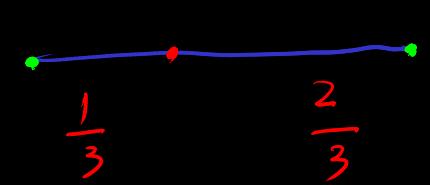
Regarding intuition, the simplest example is the proportional point of a straight line between two points
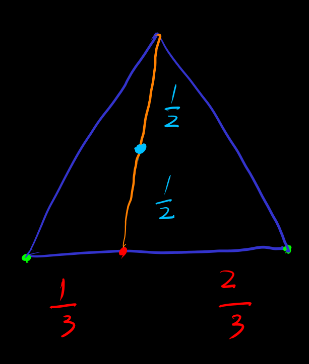
Can be iteratively or decomposed e.g. triangle . And the decomposition operation is commutative. And it can be decomposed into multiple order
[affine-coordinate] can be considered as a coordinate based on the point . Affine coordinates. alias Barycentric coordinates [barycentric-coordinate]
[affine-independent]
Affine independence := cannot be expressed as
Affine independence corresponds to the linear independence of after selecting one point e.g. as the origin
If it is affine independent, then the vertices correspond to
An -dimensional affine space has at most affine independent points
For the coordinates of affine independent points of an -dimensional affine space , have a one-to-one correspondence with the affine points of
If , although the coordinate will not change due to changing the origin, it is not an affine point
[affine-map-point-ver] alias [simplicial-map] Let be points in another affine space. The affine mapping is determined by , and the situation of other points can be obtained by generating them through affine homomorphism
[center-of-affine-point-set] The center point of is
[convex-hull] := extra
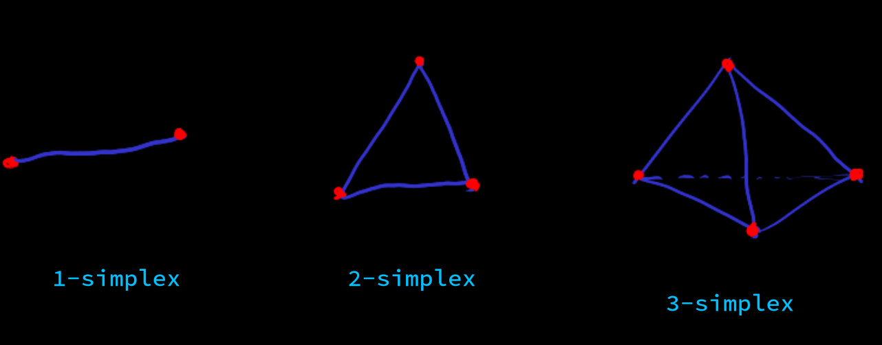
[simplex] := convex hull formed by affinely independent points
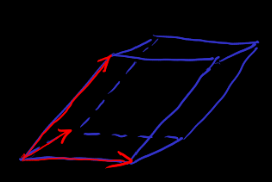
[parallelogram] Due to symmetry, the description of parallelepiped can be simplified from the convex hull of points to the description of points, after selecting the origin
[parallelogram-simplex-correspond]
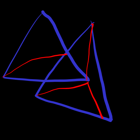
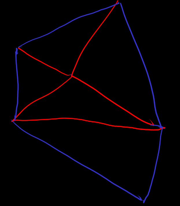
A parallelepiped can be decomposed into simplexes that are equivalent under translation and reflection (p. 587 of ref-3)
The permutations of points
Corresponding simplex
with
Conversely, a simplex also gives many parallelepipeds with it as one of the simplex blocks
The structural strength given by these two things is about the same
[volume-of-parallelogram] Volume assumption for
- Translation invariant
- Reflection invariant (unsigned volume)
- Finite (disjoint in the sense of zero measure) -> finite volume
- If are not linearly independent, then in the lower-dimensional subspace, so the -order volume is defined as zero
[volume-of-simplex] is of volume-of-parallelogram
[shear-transformation] After decomposing the parallelepiped into simplexes, cut and translate to form a new parallelepiped with the same volume. Called shear transformation. e.g.
(image from p.587 of ref-3)
Even though what we defined is the volume of a parallelepiped, the shear transformation shows that the concept of the volume of a simplex is still used simultaneously, verifying once again the close connection between simplexes and parallelepipeds
Shear transformation volume invariance is algebraically e.g. or
Scaling of edges . e.g.
The stretching and shearing of parallelepipeds corresponds to the decomposition of into elementary linear transformations, which is also used in Gaussian elimination (although they can be used for matrices)
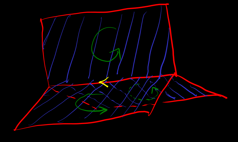
[volume-determinant] The volume change of parallelepiped is
Choose a basis of , the volume of the parallelepiped generated by it is , and the volume of other parallelepipeds is
This is the oriented volume. The set of parallelepipeds remains the same, so the absolute volume remains the same, but the directions of and are opposite
Oriented volume = Unoriented volume + Direction factor
linearly dependent ==> in a lower-dimensional subspace ==> zero volume. At this time, can be extended to , and zero volume algebraically corresponds to
For 's -th order parallelepiped and simplex
Map the parallelepiped to 's -th order alternating tensor 's decomposable element
The -multilinearity of tensors comes from the linearity of volume and side length scaling
Why is it that the concept of volume is clearly positive, yet the -alternating tensor can be negative?
Side length scaling can be extended to the direction as a form of total linearity
Any linear transformation can be decomposed into scaling and shearing. Shearing doesn't change volume, so the effect must be brought by scaling, including transformations like "swapping the order of bases," though it's not intuitively simple
Example A 2D example, but easily generalized to any two vectors in dimensions
- Shearing does not change volume
- Shearing
- Shearing
- scaling makes the volume
Actually, you could totally say it's positive multilinear alternating, positive determinant, just like the treatment of integrating densities on manifolds
[try-to-define-volume-of-low-dim] Actually, we don't need "volume invariance", we only need the volume to transform in a desirable way, that is, transform in terms of form. We don't need to define the volume of the k-th subspace of using the form of , because as long as we consider the k-th subspaces as manifolds (for example, by choosing a k-th basis to establish a coordinate system), they have their own volumes. Metric volume form is a good method to define the volume using a special family of coordinate systems in all subspaces at one time, where the metric length of is also , thus coinciding with the volume of being . For non-positive definite metric volume forms, there are some k-th subspaces where the metric length of is zero, not coinciding with the volume of being . Anyway, the following discussion may still be useful, so it is kept.
How to define low-dimensional volume? Consider two methods. Similar to linear form vs quadratic form. The first is like defining as or , the second is similar to defining or
- A basis of gives a basis of the alternating tensor space
Use it to define volume: For each , a special alternating multilinear function or form of , defined as , forall
So for a general parallelepiped the volume is
The volume of a nonzero decomposable alternating tensor can be zero, such that . The shear transformation of order does not hold for order
Question A special basis is selected, so what other bases have the same result? or what is the linear subgroup that keeps the volume unchanged?
does not preserve dimensional volume. e.g. or does not preserve dimensional volume
matrix that preserves all order volumes satisfies, for for , , or
Example (sum of elements in the th column). The and cases are similar, i.e. corresponds to the remaining sub式
(The cofactor is used in the alternating tensor decomposition representation of , which can be generalized to the alternating tensor decomposition representation or Laplace expansion of )
Example
matrix preserves all volumes satisfies
a coordinate representation of the solution
is an affine line of passing through . or is not its subset
- Select a non-degenerate quadratic form
Derive the quadratic form of the alternating space . Undirected volume or . According to the orthonormal basis and its coefficients , write it as a standard quadratic form
<==> volume is zero
In the non-Euclidean case, light-like will have an impact
Different signature volume definitions will be different for the same set of order
The two volume definitions coincide for
[convex-hull-decomposition] convex hull optimal decomposition to simplex, the method is not unique. Troublesome combinatorial problem
Example
's points
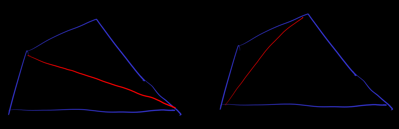
's points. First select simplex, that is, select vertices
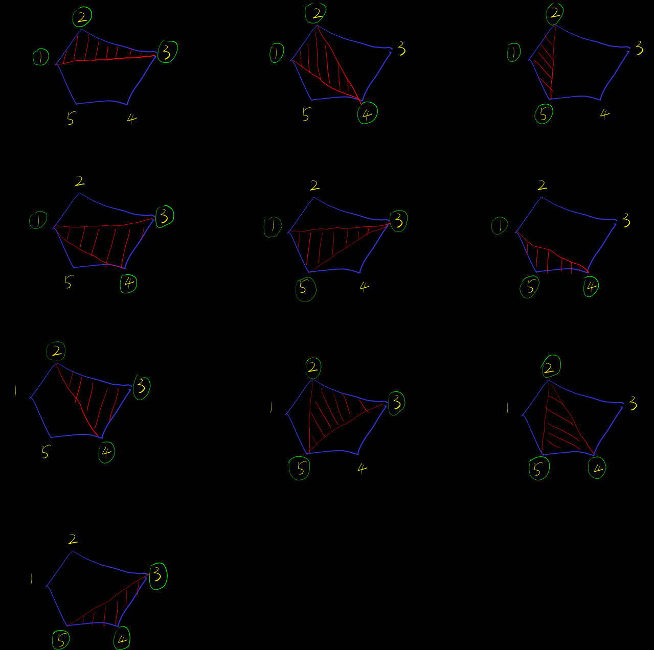
Find out which simplex combinations are decompositions of the convex hull
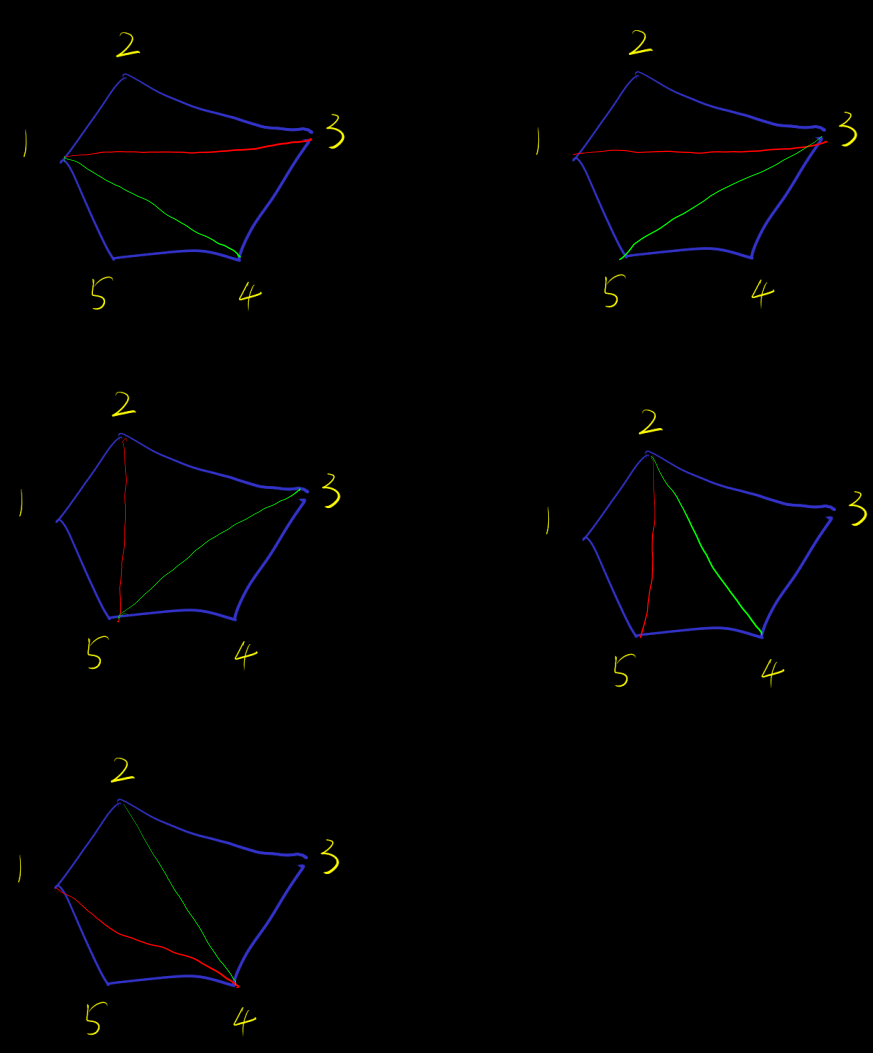
The intersection of convex hulls is a convex hull
Example
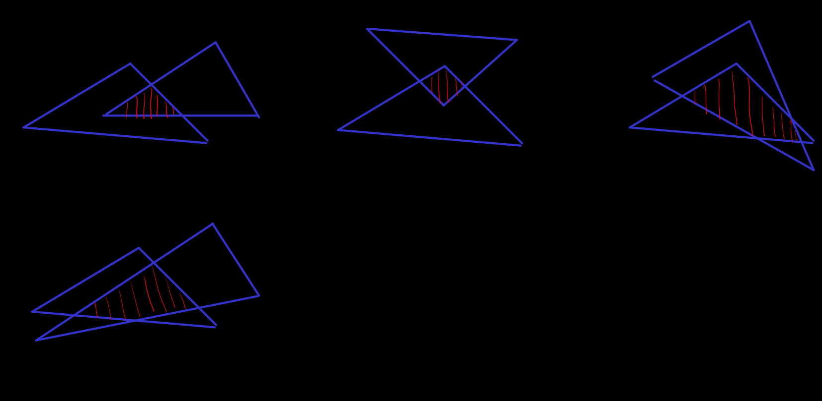
The reduced set of a simplex may not be a convex hull. But it can still be decomposed into simplex
Example
[polyhedra] Polyhedron :=
n simplex finite union with
- internally disjoint
- transitively connected between two n simplex
- the transitive boundary is n-1 simplex
The dimension of the transitive boundary is to give the polyhedron the best connectivity
[low-dim-polyhedra] Low-dimensional sub-polyhedra. As a submanifold-like setting? i.e. Adjacent simplexes with boundaries in dimension have only two -> piecewise embedded in . Otherwise, consider the example of a three-connected boundary
Countable generalization -> Countable polyhedron
[Lebesgue-measurable]
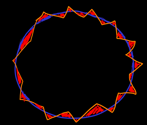
Lebesgue measurable set . Approximate with a finite union of simplex , symmetric difference cover with countable simplexes as a measure estimate error
Specifically, for a set , the outer measure is defined as if is finite. The outer measure of a polyhedron is finite, and under Euclidean distance, due to the compactness property, it can be proven to satisfy subadditivity, so the outer measure of a polyhedron is its own volume (in geometries of spaces with signatures other than Euclidean, not all polyhedra should be used to define volume).
Among sets with finite outer measure, using the outer measure of the symmetric difference as the distance , a metric space is formed (ref-12). (It is not necessary for zero distance to imply equality.) Polyhedra form a metric subspace. The volume of a polyhedron is a real-valued function on it, which can be proven to be continuous, using , the essence of the proof is using
Thus, a measurable set is defined as the closure of the family of polyhedra in the outer measure metric space. The measure of a measurable set is defined as the extension of the polyhedron volume function as a continuous function on its closure.
The definition of integration will use similar method.
Non-measurable sets are sets that have a finite outer measure but are not in the closure of polyhedra. Non-measurable sets exist (Vitali sets defined using the axiom of choice).
[Lebesgue-measure]
The symmetric difference of sets satisfies
Corresponding triangle inequality
Proof
by
The other side is similar
Triangle inequality
[try-to-define-low-dim-measure] Try to define 's dimensional measurable set. Since the codimension of the region , it is obvious that we cannot use set difference and simplex covering as measure estimation errors to approximate a general " dimensional set"
[pathologic-example-measure-of-boundary]
Using the Euclidean metric structure, some low-dimensional measurable sets can be defined, but there are still pathological examples (temporarily ignore the details, wiki it yourself)
- Painter's paradox. Measure is finite but the measure of the boundary is infinite. Unbounded region is used
- Koch snowflake. The measure is finite, but the measure of the boundary is either undefinable or infinite. Uses a boundary that is nowhere differentiable.
An example of approximating volume but not approximating the boundary volume
- Schwarz Lantern
- Infinite staircase approaching the hypotenuse of a triangle or circle ( ) or as long as there is large normal oscillation,
[measure-theoretic-boundary]
Measure theory boundary. Dimension — some supremum — may not be a natural number but a real number
For general measurable sets, intuitively, boundary =
where means that the overall scaling of a ball centered on any goes to zero
or boundary = neither inside nor outside. Inside = limit , outside = limit
Lebesgue differentiation theorem says that the measure of the boundary is zero
- The interval division of the sides of a rectangle/parallelogram gives a rectangular product-style division
- Barycentric subdivision (note that also subdivide the boundary)
