[orientation-of-real-linear-space] direction
There are two directions. for vector base of , change order once change orientable, introduce a factor. This is somewhat similar to alternating-tensor. orientation defined as quotient of vector base with same orientation. equivalent to decompose of
[orientation-of-boundary-of-simplex]
simplx oriented boundary. The direction of the boundary of simplex is to define the direction for the affine subspace where the boundary is located, such that the interior is in the -dimensional positive direction and the exterior is in the -dimensional negative direction
If we continue to define the direction for the boundary of the boundary, we will find that adjacent directions cancel out
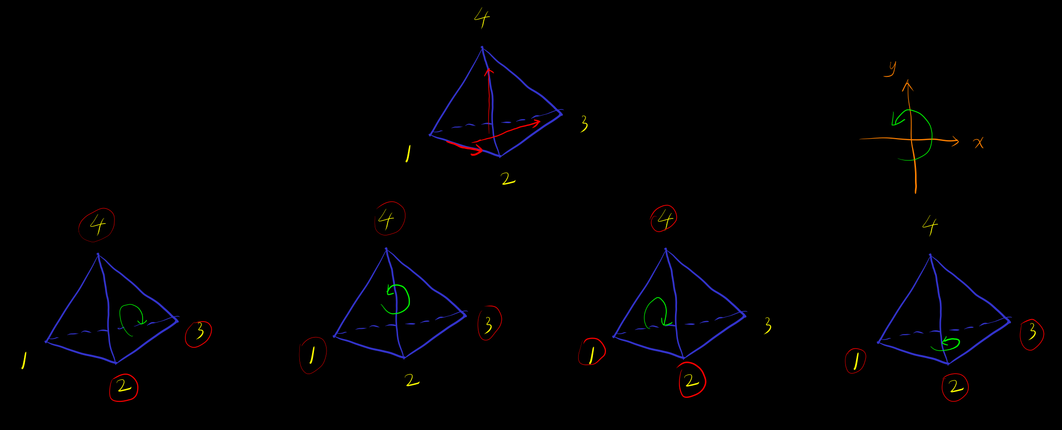
simplex vertices can construct a directed basis of according to . Permutations make the directions differ by
After selecting to be the positive direction of , the direction of the boundary is
similar to box
Example Tetrahedron, right-hand rule, with the thumb pointing towards the inside of the tetrahedron to get the boundary direction (the index of the vertices in the picture starts from instead of )
[orientable-low-dim-polyhera] Polyhedron Orientable is defined as: when constructing a polyhedron with simplexes, it is possible to define compatible orientations for all simplexes, such that the adjacent two simplexes have compatible orientations on their intersecting boundary simplexes, i.e., the orientation corresponds to the interior of simplex and the exterior of simplex . The orientation corresponds to the interior of simplex and the exterior of simplex . i.e., simplex partition has well-defined interior and exterior.
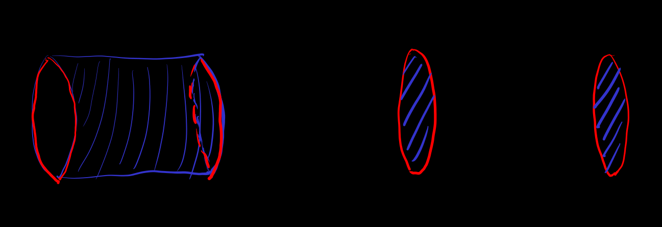
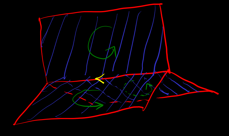
Eaxmple [Mobius-strip] Non-orientable Mobius-type polyhedron (image modified from wiki)

No matter how the direction of each simplex is defined, there exists a pair of adjacent simplex whose connected boundary simplex directions are incompatible. i.e. Simplex partitioning has no well-defined inside and outside
Starting from the initial simplex, continuously and transitively defining compatible directions for adjacent simplexes, going around in a circle will lead to incompatible directions of the connected boundary simplex. Direction corresponds to the inside of , direction corresponds to the outside of
[simplex-chain] simplex chain
[boundary-operator]
Boundary operator
boundary
Example
-
boundary-op-not-injective (p. 405 of ref-11, vol.1)

-
[tri-intersect-boundary]
cycle
or
or
[simplex-homology]
k-th homology
where are in chain space
Due to geometric meaning, only coefficients are needed
[real-linear-space-trivial-homology]
is trivial homology or or in , the boundary of is zero <==> is a boundary
Try to prove it by purely affine orientation & combinatorics technique, avoid Euclidean topology
[existence-and-uniqueness-of-n-simplex-chain-with-boundary]
in , uniqueness chain of boundary
so existence of boundary of nonzero chain
and uniqueness of dim region surround by boundary
[homology-hole] For a set minus a finite number or a countable number of separated linear subspaces or polyhedra, homology is not zero
[Stokes-theorem]
Similar to the one-dimensional Fundamental Theorem of Calculus. Intuitively, divergence and the divergence theorem = high-dimensional Fundamental Theorem of Calculus
Define [exterior-differential] in coordinates, where is the volume of the coordinates, is a large class of regions, and the calculation result does not depend on the choice of coordinates.
Then there is Stokes-theorem
for orientable analytic manifold with boundary and form with cohomology zero, or
Calculate using a box in coordinates. When all coordinates approach , it will be a partial derivative of something calculated for each coordinate axis direction. The result is , further simplification is omitted for now.
Question What is the form of the exterior derivative calculation result in the barycentric coordinates of a simplex?
However, in the proof of the one-dimensional Fundamental Theorem of Calculus, the division of a one-dimensional interval, the boundary of a one-dimensional interval, and the integral of the boundary of a one-dimensional interval are all too simple. High-dimensional regions are not that simple.
[Stokes-theorem-simple] For higher dimensions, it is difficult if it is curved. First, deal with straight things i.e. simplex or parallelepiped. The division is also the same type of region, and the boundary cancellation is also simple. Then, similar to one dimension, approximate with the Mean Value Theorem of Differential + compact control. This proves Stokes' theorem for simplex or parallelepiped.
[Stokes-theorem-proof] Question
I changed my mind. According to the intuitive treatment of integrals on manifolds and Stokes' theorem, one should use direct subdivision of the manifold, rather than approximate subdivision.
Partitioning in integration can be directly done using zero-order measurable sets (closed under diffeomorphisms). The regions used for partitioning in Stokes' theorem should be similar to sets of finite perimeter (Cacciopoli sets) in geometric measure theory (ref-33). I hope they are closed under finite unions, intersections, and subtractions, and closed under diffeomorphisms.
Prove that a manifold with boundary is locally such a region (finding polyhedral approximations based on manifold properties), and that integrals on the boundary in this theory should coincide with integrals on the boundary in manifold theory (similar to theory of reduced boundary in geometric measure theory). Prove that well-behaved manifolds with singularities also belong to such regions, i.e., polyhedra, cones, well-behaved codimensions singularity.
The proof of Stokes' theorem is to take a finite cover of compact support forms with this type of regions, subtract overlaps, partition, then use Stokes' theorem on the partitioned regions, where integrals cancel out on interior boundaries, leaving only the actual boundary of the manifold.
Although I want to avoid compact support differentiable forms, there are some cautions. the proper inclusion chain (on ) shows that, due to the lack of a differential mean value theorem, it seems that the (locally) Sobolev or absolute continuity of the form and its exterior differential is not suitable for geometrically defining the exterior differential as the limit of the boundary integral divided by the volume and then using the mean value theorem and barycentric partitioning and geometrically proving that the simplex satisfies Stokes' theorem … Although Sobolev or absolute continuity still satisfies Stokes' theorem for every local sufficient small simplex, hence if the differential is bound, we can use integral mean value to control. But mean value is the definition of Lipschitz (for simplex volume), and pure (locally) Lipschitz will also implies differential exists almost everywhere and is (locally)
As long as -dimensional affine subspaces are viewed as manifolds (for example, by choosing a -basis on them to establish a coordinate system), they have their own volume. After choosing a basis for the -subspace, the -form defined pointwise on can become real-valued on it. The integrability on the boundary of a simplex requires at least that the form becomes an integrable function in every -direction. Due to the linearity of form space and integrals, it only needs to become an integrable function on a basis of the -direction space (corresponding to the -alternating tensor space of ), which is also known as "the components of the form are locally ". At least such (locally) forms are preserved under diffeomorphisms, just as Lebesgue measurable sets are preserved under diffeomorphisms. In principle, it can be said that the function of the -subspace derived from the form in the -direction can be approximated by piecewise constant functions supported on the simplex, similar to usual integration. If we don't assume differentiable forms, then we haven't even defined the exterior derivative, nor have we proven Stokes' theorem on a simplex.
Try to define differentiation starting from integration, as a way to combine measure and differentiation. First, define what a form that satisfies the local infinitesimal Stokes' theorem is — an integrable, exterior differentiable form — and then use forms that satisfy the local infinitesimal Stokes' theorem (instead of compact support differentiable forms) to define what a region that globally satisfies Stokes' theorem is, by a polyhedral approximation.
Then try to define the exterior derivative of an form using its average derivative (using an -dimensional simplex/box/polytope/ball and its boundary shrinking to a point? The largest distance from to ) to define exterior differential.
Next, we need to prove Stokes' theorem for simplexes. Using barycentric subdivision techniques, then use estimates provided by the mean value theorem.
Then we can try to define "regions where Stokes' theorem can be applied" similar to sets of finite perimeter, or simply called sets of finite perimeter. The required restriction is that, intuitively, among all measurable sets, there is a subset of measurable sets for which the overall Stokes' theorem can be applied to their boundaries. Intuitively, the restrictions for such regions should be similar to, in the polyhedral net approximating the measurable set, there exists a sub-net that uniformly controls all normalized or projectivized integrable exterior differential forms (or something more general) on the boundary of the approximating polyhedron.
The relationship between functions of bounded variation and sets of finite perimeter in geometric measure theory is like the relationship between integrable functions and measurable sets in zero-order measure theory.
Since exterior differentiation only has first-order derivatives and there are no infinite-order exterior derivatives, on metric manifold, the norm of a form is suitable for Banach/Hilbert space theory (infinite-order derivatives are not suitable for Banach space theory).
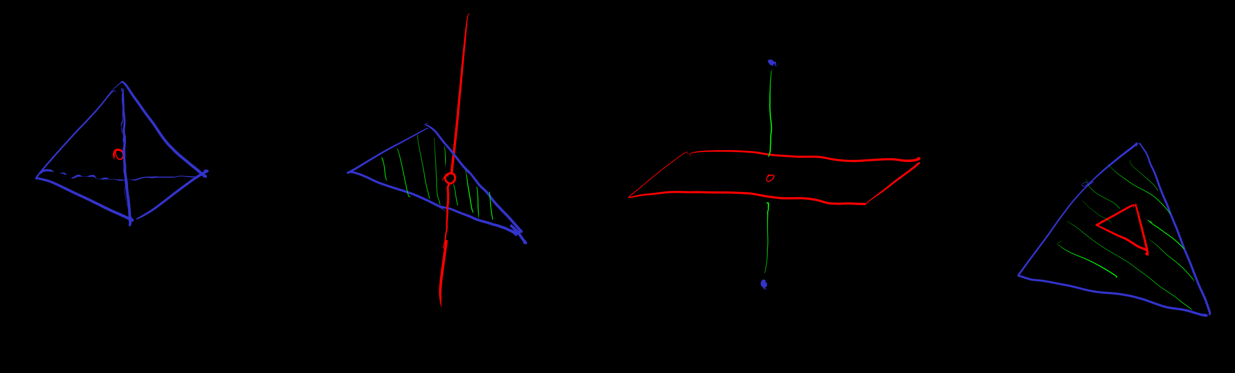
Because the topology of a manifold may have nontrivial cohomology, for some cohomologically nonzero forms , its exterior differential form cannot cancel out all internal boundaries when integral, and hence it will have some extra thing similar to "residue" in complex analysis. For example, ( [cohomology-hole] . Example In , or , satisfying , so have integral zero on , but the integral of over as the boundary of is nonzero. Example is homology isomorphism to .
Another example where the boundary integral cannot cancel out: if a vector field or form for which Stokes' theorem holds on a closed ball has a closed disk-like region on its boundary removed, Stokes' theorem no longer holds. Intuitively, after removing a closed disk, the flux leaks out, indicating that the new boundary does not enclose the interior of the manifold. If an open disk were removed instead of a closed disk, the result would not be a manifold with boundary, it would have a boundary of codimension > 1, and the boundary of the boundary would not be zero.
May need some kind of compact constraint, since non-compact will have some kind of infinity that makes boundary cancellation fail, and may have residue term
Things like the Gauss–Bonnet theorem of Euclidean metric manifold should also be provable using this method. Although it still needs to be considered why the result is a homology invariant Euler characteristic (off by an -dimensional Euclidean volume factor, expressed as a power of ) that is independent of the metric.
Todo Given counterexamples like the Cantor set construction, almost everywhere analytic is not the correct approach to handle singularity. Instead, try to use deletion of singularity to get manifold with boundary.
I have not deal with the Stokes theorem for manifold without boundary, have not define . Example of manifold without
Correspondence between boundary operator and exterior derivative
homology
cohomology
[coboundary-operator]
coboundary
cocycle . Intuitively, the divergence of the form at this point is zero
or
or
[de-Rham-cohomolgy] k-th de Rham cohomology
in , cohomology trivial
The case of metric manifolds
The integral of the form is equivalent to the integral of
[Hodge-star]
Hodge star operator as the orthogonal complement dual of the form
with ==>
==>
[flux]
Integral of form -> Integral of -> Integral of , interpreted as the quantity of the orthogonal complement of integrated over , i.e. flux
Represent the flux alternating tensor using the inner product duality , the inner product represents the orthogonal projection of the quantity onto the flux direction (image)
Example in Euclidean , .
- form
Coordinates
Stokes' theorem [gradient]
- form
Note that at this time, you can add a directional two-dimensional "rotation 90 degrees" to change the two-dimensional divergence into a two-dimensional curl, and the normal flux to the boundary becomes the tangent flow to the boundary.
Coordinates
Stokes' Theorem [curl]
where
- form
Coordinates
Stokes' Theorem [divergence]
in Minkowski ,